How to Construct Splines

Open Live Script

This example shows how to construct splines in various ways using the spline functions in Curve Fitting Toolbox™.

Interpolation

你可以建立一个立方样条插值that matches the cosine function at the following sitesX，使用CSAPI命令。

X= 2*pi*[0 1 .1:.2:.9]; y = cos(x); cs = csapi(x,y);

You can then view the interpolating spline by usingfnplt。

fnplt(cs,2); axis([-1 7 -1.2 1.2]) holdonplot(x,y,'o') holdoff

图包含一个坐标轴对象。坐标轴对象有限公司ntains 2 objects of type line.

检查插值

余弦函数为2*pi-periodic。在这方面，我们的立方样条插值的表现如何？检查的一种方法是在两个端点处计算第一个衍生物中的差异。

diff( fnval( fnder(cs), [0 2*pi] ) )

ANS = -0.1375

要执行周期性，请使用csape代替CSAPI。

csp = csape (x,y,“周期性”）；抓住onFNPLT（CSP，'g') holdoff

图包含一个坐标轴对象。轴对象包含3个类型行的对象。

现在检查给

diff（fnval（fnder（csp），[0 2*pi]））

ans = -2.2806e-17

Even the second derivative now matches at the endpoints.

diff（fnval（fnder（csp，2），[0 2*pi]））

ANS = -2.2204E -16

这piecewise linear interpolantto the same data is available viaSPAPI。在这里，我们将其添加到先前的图中，红色。

pl = spapi（2，x，y）;抓住onfnplt(pl,'r'，，，，2) holdoff

图包含一个坐标轴对象。坐标轴对象有限公司ntains 4 objects of type line.

Smoothing

If the data are noisy, you usually want to approximate rather than interpolate. For example, with these data

X= linspace(0,2*pi,51); noisy_y = cos(x) + .2*(rand(size(x))-.5); plot(x,noisy_y,'x'）轴（[-1 7 -1.2 1.2]）

图包含一个坐标轴对象。坐标轴对象有限公司ntains an object of type line.

插值将使下面以蓝色显示wiggly interpolant。

抓住onfnplt( csapi(x, noisy_y) ) holdoff

图包含一个坐标轴对象。坐标轴对象有限公司ntains 2 objects of type line.

In contrast, smoothing with a proper tolerance

tol =（.05）^2*（2*pi）

tol = 0.0157

给出平滑的近似值，如下所示。

抓住onfnplt( spaps(x, noisy_y, tol),'r'，2）保持off

图包含一个坐标轴对象。轴对象包含3个类型行的对象。

近似值在间隔的末端附近要差得多，并且远非周期性。为了执行周期性，将近似于定期扩展的数据，然后将近似值限制为原始间隔。

noisy_y([1 end]) = mean( noisy_y([1 end]) ); lx = length(x); lx2 = round(lx/2); range = [lx2:lx 2:lx 2:lx2]; sps = spaps([x(lx2:lx)-2*pi x(2:lx) x(2:lx2)+2*pi],noisy_y(range),2*tol);

This gives the more nearly periodic approximation, shown in black.

抓住onfnplt(sps, [0 2*pi],'k'，，，，2) holdoff

图包含一个坐标轴对象。坐标轴对象有限公司ntains 4 objects of type line.

最小二乘近似

另外，您可以通过几样的自由度来对噪声数据使用最小二乘近似。

For example, you might try a cubic spline with just four pieces.

spl2 = spap2（4，4，x，noisy_y）;fnplt（spl2，'b'，2）;轴（[ -  1 7 -1.2 1.2]）onplot(x,noisy_y,'x') holdoff

图包含一个坐标轴对象。坐标轴对象有限公司ntains 2 objects of type line.

Knot Selection

When usingSPAPIorSPAP2，您通常必须指定特定的样条空间。这是通过指定一个结序列和order，这可能有点问题。但是，在进行样条插值时x，y使用订单样条的数据k，，，，you can use the functionOPTKNT如下示例，要提供一个好的结序。

k= 5;% order 5, i.e., we are working with quartic splinesX= 2*pi*sort([0 1 rand(1,10)]); y = cos(x); sp = spapi( optknt(x,k), x, y ); fnplt(sp,2,'g'）；抓住onplot(x,y,'o') holdoff轴（[ -  1 7 -1.1 1.1]）

图包含一个坐标轴对象。坐标轴对象有限公司ntains 2 objects of type line.

进行最小二乘近似时，您可以使用当前近似值来确定可能更好的结选择newknt。例如，以下对指数函数的近似并不是那么好，从其误差中可以看出，以红色绘制。

X= linspace(0,10,101); y = exp(x); sp0 = spap2( augknt(0:2:10,4), 4, x, y ); plot(x,y-fnval(sp0,x),'r'，，，，'LineWidth'，，，，2)

图包含一个坐标轴对象。坐标轴对象有限公司ntains an object of type line.

但是，您可以使用该初始近似来与相同的number of knots, but which are better distributed. Its error is plotted in black.

sp1 = spap2( newknt(sp0), 4, x, y ); holdon图（x，y-fnval（sp1，x），'k'，，，，'LineWidth'，2）保持off

图包含一个坐标轴对象。坐标轴对象有限公司ntains 2 objects of type line.

Gridded Data

All the spline interpolation and approximation commands in the Curve Fitting Toolbox can also handle gridded data, in any number of variables.

For example, here is a bicubic spline interpolant to the Mexican Hat function.

X=.0001+(-4:.2:4); y = -3:.2:3; [yy,xx] = meshgrid(y,x); r = pi*sqrt(xx.^2+yy.^2); z = sin(r)./r; bcs = csapi({x,y}, z); fnplt(bcs) axis([-5 5 -5 5 -.5 1])

图包含一个坐标轴对象。轴对象包含类型表面的对象。

Here is theleast-squares同一网格上同一函数的噪声值的近似值。

knotsx = augknt（linspace（x（1），x（end），21），4）;knotsy = augknt（linspace（y（1），y（end），15），4）;bsp2 = spap2（{knotsx，knotsy}，[4 4]，{x，y}，z+.02*（rand（size（z）） -  .5））;FNPLT（BSP2）轴（[-5 5 -5 5 -.5 1]）

图包含一个坐标轴对象。轴对象包含类型表面的对象。

Curves

网格数据可以轻松处理，因为曲线拟合工具箱可以处理矢量值splines. This also makes it easy to work with parametric curves.

Here, for example, is an approximation to infinity, obtained by putting a cubic spline curve through the points marked in the following figure.

t = 0：8;xy = [0 0; 1 1;1.7 0; 1 -1; 0 0;-1 1;-1.7 0;-1 -1;0 0]。';infty = csape（t，xy，“周期性”）；fnplt（Infty，2）轴（[-2 2 -2 -1.1 1.1]）保持onplot(xy(1,:),xy(2,:),'o') holdoff

图包含一个坐标轴对象。坐标轴对象有限公司ntains 2 objects of type line.

Here is the same curve, but with motion in a third dimension.

roller = csape( t , [ xy ;0 1/2 1 1/2 0 1/2 1 1/2 0],“周期性”）；fnplt（滚子，2，[0 4]，，'b') holdonfnplt（滚子，2，[4 8]，，'r'）plot3（0,0,0，'o') holdoff

图包含一个坐标轴对象。轴对象包含3个类型行的对象。

这two halves of the curve are plotted in different colors and the origin is marked, as an aid to visualizing this two-winged space curve.

表面

带有R^3中值的双变量张量产物样条具有表面。例如，这是圆环的良好近似值。

X= 0:4; y = -2:2; R = 4; r = 2; v = zeros(3,5,5); v(3,:,:) = [0 (R-r)/2 0 (r-R)/2 0].'*[1 1 1 1 1]; v(2,:,:) = [R (r+R)/2 r (r+R)/2 R].'*[0 1 0 -1 0]; v(1,:,:) = [R (r+R)/2 r (r+R)/2 R].'*[1 0 -1 0 1]; dough0 = csape({x,y},v,“周期性”）；fnplt(dough0) axis平等的，轴off

这是该表面的正常冠。

nx = 43; xy = [ones(1,nx); linspace(2,-2,nx)]; points = fnval(dough0,xy)'; ders = fnval(fndir(dough0,eye(2)),xy); normals = cross(ders(4:6,:),ders(1:3,:)); normals = (normals./repmat(sqrt(sum(normals.*normals)),3,1))'; pn = [points;points+normals]; holdon为了j=1:nx plot3(pn([j,j+nx],1),pn([j,j+nx],2),pn([j,j+nx],3))结尾抓住off

Finally, here is its projection onto the (x,y)-plane.

fnplt（fncmb（面团，[1 0 0; 0 1 0]））轴（[ -  5.25 5.25 -4.14 4.14]），轴off

Scattered Data

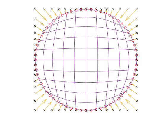
也可以插入平面中未播种数据位点给出的值。例如，考虑将单元正方形平滑映射到设备磁盘的任务。我们构建标记为圆圈的数据值和标记为X的相应数据站点。每个数据站点通过箭头连接到其关联的值。

n = 64; t = linspace(0,2*pi,n+1); t(end) = []; values = [cos(t); sin(t)]; plot(values(1,:),values(2,:),'or'）轴平等的，轴offsites = values./repmat(max(abs(values)),2,1); holdon绘图（站点（1，:)，站点（2，2 ：），，，'xk'）Quiver（站点（1，:)，站点（2，2 :)，，，...values(1,:)-sites(1,:), values(2,:)-sites(2,:)) holdoff

然后使用TPAP构建双变量插值矢量值薄板样条。

英石= tpaps(sites, values, 1);

样条确实确实平稳地绘制了单位正方形（大约）到设备磁盘，作为其图的图fnplt指示。该图显示了在样条图下均匀间隔的平方网格的图像英石。

抓住onfnplt（st）保持off