Set Up Your Mobile Device

In order to receive data from a mobile device in MATLAB®, you will need to install and set up the MATLAB Mobile™ app on your mobile device.

Log in to the MathWorks® Cloud from the MATLAB Mobile Settings.

Create a Connection to Your Mobile Device

On theCommandsscreen of MATLAB Mobile, use themobiledevcommand to create an object that represents your mobile device.

m = mobiledev;

The displayed output should showConnected: 1, indicating that themobiledevobject has successfully established a connection to the app.

Prepare for Data Acquisition from the Position Sensor

In order to collect GPS data, first ensure that your device's GPS is turned on. If enabled on the mobile device's location settings, mobile networks and Wi-Fi can also be used to determine position.

Enable the position sensor on your mobile device.

m.PositionSensorEnabled = 1;

It may take some time for data to appear on theSensorsscreen of MATLAB Mobile, as the device will need to search for a GPS signal. GPS signals are generally unavailable indoors.

Start Acquiring Data

一个fter enabling the sensors, theSensorsscreen of MATLAB Mobile will show the current data measured by the sensors. TheLoggingproperty allows you to begin sending sensor data tomobiledev.

m.Logging = 1;

Gather Position Data

一个ll position sensor data recorded on the device is now being logged bymobiledev.

In this example, the device was taken on a short drive around MathWorks.

Stop Logging Data

Usemobiledev's logging property again to stop logging data.

m.Logging = 0;

Retrieve Logged Position Data

To create the map, latitude, longitude, and speed data will be needed. Theposlogfunction can be used to retrieve this information frommobiledev.

[lat,lon,t,spd] = poslog(m);

For this example, data has already been logged and saved.

loaddrivingAroundMathWorkslatlonspd;

Bin Speeds into Color Values

The speed values are binned in order to use a discrete number of colors to represent the observed speeds.

nBins = 10; binSpacing = (max(spd) - min(spd))/nBins; binRanges = min(spd):binSpacing:max(spd)-binSpacing;% Add an inf to binRanges to enclose the values above the last bin.binRanges(end+1) = inf;% |histc| determines which bin each speed value falls into.[~, spdBins] = histc(spd, binRanges);

Split Latitude and Longitude Data by Speed

一个discontinuous line segment is created for every speed bin. Each of these segments will be assigned a single color. This creates far fewer total line segments than treating every adjacent pair of latitude and longitude values as their own line segments.

The individual segments are stored as geographic features usinggeoshapefrom Mapping Toolbox.

lat = lat'; lon = lon'; spdBins = spdBins';% Create a geographical shape vector, which stores the line segments as% features.s = geoshape();fork = 1:nBins% Keep only the lat/lon values which match the current bin. Leave the% rest as NaN, which are interpreted as breaks in the line segments.latValid = nan(1, length(lat)); latValid(spdBins==k) = lat(spdBins==k); lonValid = nan(1, length(lon)); lonValid(spdBins==k) = lon(spdBins==k);% To make the path continuous despite being segmented into different% colors, the lat/lon values that occur after transitioning from the% current speed bin to another speed bin will need to be kept.transitions = [diff(spdBins) 0]; insertionInd = find(spdBins==k & transitions~=0) + 1;% Preallocate space for and insert the extra lat/lon values.latSeg = 0(1、长度(latValid) +(插入长度ionInd)); latSeg(insertionInd + (0:length(insertionInd)-1)) = lat(insertionInd); latSeg(~latSeg) = latValid; lonSeg = zeros(1, length(lonValid) + length(insertionInd)); lonSeg(insertionInd + (0:length(insertionInd)-1)) = lon(insertionInd); lonSeg(~lonSeg) = lonValid;% Add the lat/lon segments to the geographic shape vector.s(k) = geoshape(latSeg, lonSeg);end

Create a Web Map and Route Overlay

The pieces can now be combined into a webmap display. The latitude and longitude data have been processed to make up individual line segments to overlay on the map. Each line segment has a color corresponding to the speed recorded at the respective position.

Mapping Toolbox provides a number of functions for working with web maps.

Usewebmapto open a web map in a browser.

wm = webmap('Open Street Map');

For reference, MathWorks is marked on the map.

mwLat = 42.299827; mwLon = -71.350273; name ='MathWorks'; iconDir = fullfile(matlabroot,'toolbox','matlab','icons'); iconFilename = fullfile(iconDir,'matlabicon.gif'); wmmarker(mwLat, mwLon,'FeatureName', name,'Icon', iconFilename);

一个list of colors corresponding to the speed bins is generated using theautumncolormap. This creates an[nBins x 3]matrix with RGB values for each bin.

colors = autumn(nBins);

一个line is drawn on the webmap using the geographic shape vector. Each element of the shape vector corresponds to a discontinuous line segment for a binned speed value. These elements match the elements of the color list that was just created.

wmline(s,'Color', colors,'Width', 5);

Zoom the map in on the route.

wmzoom(16);

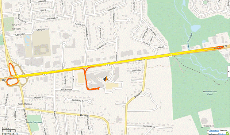
The final display provides a visual representation of location and speed throughout the route. The device was clearly traveling more slowly while in the parking lot and during turns than it was on straightaways.

Clean Up

关闭位置传感器和明确的mobiledev.

m.PositionSensorEnabled = 0; clearm;