Constrained Electrostatic Nonlinear Optimization, Problem-Based

Open Live Script

Consider the electrostatics problem of placing 20 electrons in a conducting body. The electrons will arrange themselves in a way that minimizes their total potential energy, subject to the constraint of lying inside the body. All the electrons are on the boundary of the body at a minimum. The electrons are indistinguishable, so the problem has no unique minimum (permuting the electrons in one solution gives another valid solution). This example was inspired by Dolan, Moré, and Munson [1].

The objective and nonlinear constraint functions for this example are allSupported Operations for Optimization Variables and Expressions. Therefore,solveuses automatic differentiation to calculate gradients. SeeAutomatic Differentiation in Optimization Toolbox. Without automatic differentiation, this example stops early by reaching theMaxFunctionEvaluationstolerance. For an equivalent solver-based example using Symbolic Math Toolbox™, seeCalculate Gradients and Hessians Using Symbolic Math Toolbox.

Problem Geometry

This example involves a conducting body defined by the following inequalities. For each electron with coordinates $(x, y, z)$ ,

$\begin{array}{l} z \leq - | x | - | y | \\ x^{2} + y^{2} + (z + 1)^{2} \leq 1 . \end{array}$

These constraints form a body that looks like a pyramid on a sphere. To view the body, enter the following code.

[X,Y] = meshgrid(-1:.01:1); Z1 = -abs(X) - abs(Y); Z2 = -1 - sqrt(1 - X.^2 - Y.^2); Z2 = real(Z2); W1 = Z1; W2 = Z2; W1(Z1 < Z2) = nan;% Only plot points where Z1 > Z2W2 (Z1 < Z2) =南;% Only plot points where Z1 > Z2hand = figure;% Handle to the figure, for later useset(gcf,'Color','w')% White backgroundsurf(X,Y,W1,'LineStyle','none'); holdonsurf(X,Y,W2,'LineStyle','none'); view(-44,18)

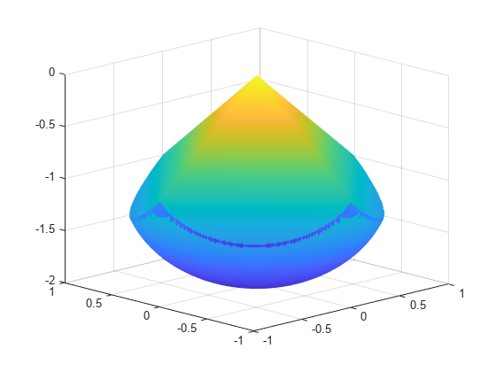
Figure contains an axes object. The axes object contains 2 objects of type surface.

A slight gap exists between the upper and lower surfaces of the figure. This gap is an artifact of the general plotting routine used to create the figure. The routine erases any rectangular patch on one surface that touches the other surface.

Define Problem Variables

The problem has twenty electrons. The constraints give bounds on each $x$ and $y$ value from –1 to 1, and the $z$ 值从2到0。定义variables for the problem.

N = 20; x = optimvar('x',N,'LowerBound',-1,'UpperBound',1); y = optimvar('y',N,'LowerBound',-1,'UpperBound',1); z = optimvar('z',N,'LowerBound',-2,'UpperBound',0); elecprob = optimproblem;

Define Constraints

The problem has two types of constraints. The first, a spherical constraint, is a simple polynomial inequality for each electron separately. Define this spherical constraint.

elecprob.Constraints.spherec = (x.^2 + y.^2 + (z+1).^2) <= 1;

The preceding constraint command creates a vector of ten constraints. View the constraint vector usingshow.

show(elecprob.Constraints.spherec)

((x.^2 + y.^2) + (z + 1).^2) <= arg_RHS where: arg2 = 1; arg1 = arg2(ones(1,20)); arg_RHS = arg1(:);

The second type of constraint in the problem is linear. You can express the linear constraints in different ways. For example, you can use theabsfunction to represent an absolute value constraint. To express the constraints this way, write a MATLAB function and convert it to an expression usingfcn2optimexpr. SeeConvert Nonlinear Function to Optimization Expression. For a preferable approach that uses only differentiable functions, write the absolute value constraint as four linear inequalities. Each constraint command returns a vector of 20 constraints.

elecprob.Constraints.plane1 = z <= -x-y; elecprob.Constraints.plane2 = z <= -x+y; elecprob.Constraints.plane3 = z <= x-y; elecprob.Constraints.plane4 = z <= x+y;

Define Objective Function

The objective function is the potential energy of the system, which is a sum over each electron pair of the inverse of their distances:

$e n e r g y = \sum_{i < j} \frac{1}{‖ e l e c t r o n (i) - e l e c t r o n (j) ‖} .$

定义objective function as an optimization expression. For good performance, write the objective function in a vectorized fashion. SeeCreate Efficient Optimization Problems.

energy = optimexpr(1);forii = 1:(N-1) jj = (ii+1):N; tempe = (x(ii) - x(jj)).^2 + (y(ii) - y(jj)).^2 + (z(ii) - z(jj)).^2; energy = energy + sum(tempe.^(-1/2));endelecprob.Objective = energy;

Run Optimization

Start the optimization with the electrons distributed randomly on a sphere of radius 1/2 centered at [0,0,–1].

rngdefault% For reproducibilityx0 = randn(N,3);forii=1:N x0(ii,:) = x0(ii,:)/norm(x0(ii,:))/2; x0(ii,3) = x0(ii,3) - 1;endinit.x = x0(:,1); init.y = x0(:,2); init.z = x0(:,3);

Solve the problem by callingsolve.

[sol,fval,exitflag,output] = solve(elecprob,init)

使用fmincon解决问题。发现局部最小值that satisfies the constraints. Optimization completed because the objective function is non-decreasing in feasible directions, to within the value of the optimality tolerance, and constraints are satisfied to within the value of the constraint tolerance.

sol =struct with fields:x: [20x1 double] y: [20x1 double] z: [20x1 double]

fval = 163.0099

exitflag = OptimalSolution

output =struct with fields:iterations: 94 funcCount: 150 constrviolation: 0 stepsize: 2.8395e-05 algorithm: 'interior-point' firstorderopt: 8.1308e-06 cgiterations: 0 message: 'Local minimum found that satisfies the constraints....' bestfeasible: [1x1 struct] objectivederivative: "reverse-AD" constraintderivative: "closed-form" solver: 'fmincon'

View Solution

Plot the solution as points on the conducting body.

figure(hand) plot3(sol.x,sol.y,sol.z,'r.','MarkerSize',25) holdoff

Figure contains an axes object. The axes object contains 3 objects of type surface, line.

The electrons are distributed fairly evenly on the constraint boundary. Many electrons are on the edges and the pyramid point.

Reference

[1] Dolan, Elizabeth D., Jorge J. Moré, and Todd S. Munson. “Benchmarking Optimization Software with COPS 3.0.” Argonne National Laboratory Technical Report ANL/MCS-TM-273, February 2004.