Gauss-Laguerre Quadrature Evaluation Points and Weights

Open Live Script

This example shows how to solve polynomial equations and systems of equations, and work with the results using Symbolic Math Toolbox™.

Gaussian quadrature rules approximate an integral by sums $\int_{a}^{b} f (t) w (t) d t \approx \sum_{i = 1}^{n} f (x_{i}) α_{i}$ . Here, the $x_{i}$ and $α_{i}$ are parameters of the method, depending on $n$ but not on $f$ . They follow from the choice of the weight function $w (t)$ , as follows. Associated to the weight function is a family of orthogonal polynomials. The polynomials' roots are the evaluation points $x_{i}$ . Finally, the weights $α_{i}$ are determined by the condition that the method be correct for polynomials of small degree. Consider the weight function $w (t) = \exp (- t)$ on the interval $[0, \infty]$ . This case is known as Gauss-Laguerre quadrature.

symstn = 4; w(t) = exp(-t);

Assume you know the first $n$ members of the family of orthogonal polynomials. In case of the quadrature rule considered here, they turn out to be the Laguerre polynomials.

F = laguerreL(0:n-1, t)

F =
                 
                   $(\begin{array}{c} 1 & 1 - t & \frac{t^{2}}{2} - 2 t + 1 & - \frac{t^{3}}{6} + \frac{3 t^{2}}{2} - 3 t + 1 \end{array})$

LetLbe the $n + 1$ st polynomial, the coefficients of which are still to be determined.

X = sym('X', [1, n+1])

X =
                  $(\begin{array}{c} X_{1} & X_{2} & X_{3} & X_{4} & X_{5} \end{array})$

L = poly2sym(X, t)

L =
                  $X_{1} t^{4} + X_{2} t^{3} + X_{3} t^{2} + X_{4} t + X_{5}$

Represent the orthogonality relations between the Laguerre polynomialsFandLin a system of equationssys.

sys = [int(F.*L.*w(t), t, 0, inf) == 0]

sys =
                  $(\begin{array}{c} 24 X_{1} + 6 X_{2} + 2 X_{3} + X_{4} + X_{5} = 0 & - 96 X_{1} - 18 X_{2} - 4 X_{3} - X_{4} = 0 & 144 X_{1} + 18 X_{2} + 2 X_{3} = 0 & - 96 X_{1} - 6 X_{2} = 0 \end{array})$

Add the condition that the polynomial have norm 1.

sys = [sys, int(L^2.*w(t), 0, inf) == 1]

sys =
                  $(\begin{array}{c} 24 X_{1} + 6 X_{2} + 2 X_{3} + X_{4} + X_{5} = 0 & - 96 X_{1} - 18 X_{2} - 4 X_{3} - X_{4} = 0 & 144 X_{1} + 18 X_{2} + 2 X_{3} = 0 & - 96 X_{1} - 6 X_{2} = 0 & 40320 {X_{1}}^{2} + 10080 X_{1} X_{2} + 1440 X_{1} X_{3} + 240 X_{1} X_{4} + 48 X_{1} X_{5} + 720 {X_{2}}^{2} + 240 X_{2} X_{3} + 48 X_{2} X_{4} + 12 X_{2} X_{5} + 24 {X_{3}}^{2} + 12 X_{3} X_{4} + 4 X_{3} X_{5} + 2 {X_{4}}^{2} + 2 X_{4} X_{5} + {X_{5}}^{2} = 1 \end{array})$

Solve for the coefficients ofL.

S = solve(sys, X)

S =结构体字段:X1: [2x1 sym] X2: [2x1 sym] X3: [2x1 sym] X4: [2x1 sym] X5: [2x1 sym]

solvereturns the two solutions in a structure array. Display the solutions.

structfun(@display, S)

ans =
                 
                   $(\begin{array}{c} - \frac{1}{24} \\ \frac{1}{24} \end{array})$

ans =
                 
                   $(\begin{array}{c} \frac{2}{3} \\ - \frac{2}{3} \end{array})$

ans =
                 
                   $(\begin{array}{c} - 3 \\ 3 \end{array})$

ans =
                 
                   $(\begin{array}{c} 4 \\ - 4 \end{array})$

ans =
                 
                   $(\begin{array}{c} - 1 \\ 1 \end{array})$

Make the solution unique by imposing an extra condition that the first coefficient be positive:

sys = [sys, X(1)>0]; S = solve(sys, X)

S =结构体字段:X1: 1/24 X2: -2/3 X3: 3 X4: -4 X5: 1

Substitute the solution intoL.

L = subs(L, S)

L =
                 
                   $\frac{t^{4}}{24} - \frac{2 t^{3}}{3} + 3 t^{2} - 4 t + 1$

As expected, this polynomial is the |n|th Laguerre polynomial:

laguerreL(n, t)

ans =
                 
                   $\frac{t^{4}}{24} - \frac{2 t^{3}}{3} + 3 t^{2} - 4 t + 1$

The evaluation points $x_{i}$ are the roots of the polynomialL. SolveLfor the evaluation points. The roots are expressed in terms of therootfunction.

x = solve(L)

x =
                 
                   $\begin{array}{l} (\begin{array}{c} root (σ_{1}, z, 1) \\ root (σ_{1}, z, 2) \\ root (σ_{1}, z, 3) \\ root (σ_{1}, z, 4) \end{array}) \\ where \\ σ_{1} = z^{4} - 16 z^{3} + 72 z^{2} - 96 z + 24 \end{array}$

The form of the solutions might suggest that nothing has been achieved, but various operations are available on them. Compute floating-point approximations usingvpa:

vpa(x)

ans =
                 
                   $(\begin{array}{c} 0.32254768961939231180036145910437 \\ 1.7457611011583465756868167125179 \\ 4.5366202969211279832792853849571 \\ 9.3950709123011331292335364434205 \end{array})$

Some spurious imaginary parts might occur. Prove symbolically that the roots are real numbers:

isAlways(in(x,'real'))

ans =4x1 logical array1 1 1 1

For polynomials of degree less than or equal to 4, you can useMaxDegreeto obtain the solutions in terms of nested radicals instead in terms ofroot. However, subsequent operations on results of this form would be slow.

xradical = solve(L,'MaxDegree', 4)

xradical =
                 
                   $\begin{array}{l} (\begin{array}{c} 4 - σ_{1} - σ_{3} \\ 4 + σ_{1} - σ_{3} \\ σ_{3} - σ_{2} + 4 \\ σ_{3} + σ_{2} + 4 \end{array}) \\ where \\ σ_{1} = \frac{\sqrt{96 σ_{6} σ_{4} - 3 σ_{5} σ_{4} - 288 σ_{4} - 512 \sqrt{3} \sqrt{6} \sqrt{6 + \sqrt{3} \sqrt{6} i}}}{2 {(768 + 128 \sqrt{3} \sqrt{6} i)}^{1 / 6} {(144 σ_{6} + 9 σ_{5} + 864)}^{1 / 4}} \\ σ_{2} = \frac{\sqrt{96 σ_{6} σ_{4} - 3 σ_{5} σ_{4} - 288 σ_{4} + 512 \sqrt{3} \sqrt{6} \sqrt{6 + \sqrt{3} \sqrt{6} i}}}{2 {(768 + 128 \sqrt{3} \sqrt{6} i)}^{1 / 6} {(144 σ_{6} + 9 σ_{5} + 864)}^{1 / 4}} \\ σ_{3} = \frac{σ_{4}}{2 {(768 + 128 \sqrt{3} \sqrt{6} i)}^{1 / 6}} \\ σ_{4} = \sqrt{16 σ_{6} + σ_{5} + 96} \\ σ_{5} = {(768 + 128 \sqrt{3} \sqrt{6} i)}^{2 / 3} \\ σ_{6} = {(768 + 128 \sqrt{3} \sqrt{6} i)}^{1 / 3} \end{array}$

The weights $α_{i}$ are given by the condition that for polynomials of degree less than $n$ , the quadrature rule must produce exact results. It is sufficient if this holds for a basis of the vector space of these polynomials. This condition results in a system of four equations in four variables.

y = sym('y', [n, 1]); sys = sym(zeros(n));fork=0:n-1 sys(k+1) = sum(y.*(x.^k)) == int(t^k * w(t), t, 0, inf);endsys

sys =
                 
                   $\begin{array}{l} (\begin{array}{c} y_{1} + y_{2} + y_{3} + y_{4} = 1 & 0 & 0 & 0 \\ y_{1} root (σ_{1}, z, 1) + y_{2} root (σ_{1}, z, 2) + y_{3} root (σ_{1}, z, 3) + y_{4} root (σ_{1}, z, 4) = 1 & 0 & 0 & 0 \\ y_{1} {root (σ_{1}, z, 1)}^{2} + y_{2} {root (σ_{1}, z, 2)}^{2} + y_{3} {root (σ_{1}, z, 3)}^{2} + y_{4} {root (σ_{1}, z, 4)}^{2} = 2 & 0 & 0 & 0 \\ y_{1} {root (σ_{1}, z, 1)}^{3} + y_{2} {root (σ_{1}, z, 2)}^{3} + y_{3} {root (σ_{1}, z, 3)}^{3} + y_{4} {root (σ_{1}, z, 4)}^{3} = 6 & 0 & 0 & 0 \end{array}) \\ where \\ σ_{1} = z^{4} - 16 z^{3} + 72 z^{2} - 96 z + 24 \end{array}$

Solve the system both numerically and symbolically. The solution is the desired vector of weights $α_{i}$ .

[a1, a2, a3, a4] = vpasolve(sys, y)

a1 =
                  $0.60315410434163360163596602381808$

a2 =
                  $0.35741869243779968664149201745809$

a3 =
                  $0.03888790851500538427243816815621$

a4 =
                  $0.00053929470556132745010379056762059$

[alpha1, alpha2, alpha3, alpha4] = solve(sys, y)

alpha1 =
                 
                   $\begin{array}{l} - \frac{σ_{3} σ_{2} + σ_{3} σ_{1} + σ_{2} σ_{1} - σ_{3} σ_{2} σ_{1} - 2 σ_{3} - 2 σ_{2} - 2 σ_{1} + 6}{(σ_{4} - σ_{3}) (σ_{4} σ_{2} + σ_{4} σ_{1} - σ_{2} σ_{1} - {σ_{4}}^{2})} \\ where \\ σ_{1} = root (z^{4} - 16 z^{3} + 72 z^{2} - 96 z + 24, z, 4) \\ σ_{2} = root (z^{4} - 16 z^{3} + 72 z^{2} - 96 z + 24, z, 3) \\ σ_{3} = root (z^{4} - 16 z^{3} + 72 z^{2} - 96 z + 24, z, 2) \\ σ_{4} = root (z^{4} - 16 z^{3} + 72 z^{2} - 96 z + 24, z, 1) \end{array}$

alpha2 =
                 
                   $\begin{array}{l} \frac{root (σ_{1}, z, 1) root (σ_{1}, z, 3) + root (σ_{1}, z, 1) root (σ_{1}, z, 4) + root (σ_{1}, z, 3) root (σ_{1}, z, 4) - root (σ_{1}, z, 1) root (σ_{1}, z, 3) root (σ_{1}, z, 4) - 2 root (σ_{1}, z, 1) - 2 root (σ_{1}, z, 3) - 2 root (σ_{1}, z, 4) + 6}{(root (σ_{1}, z, 2) - root (σ_{1}, z, 1)) (root (σ_{1}, z, 2) - root (σ_{1}, z, 3)) (root (σ_{1}, z, 2) - root (σ_{1}, z, 4))} \\ where \\ σ_{1} = z^{4} - 16 z^{3} + 72 z^{2} - 96 z + 24 \end{array}$

alpha3 =
                 
                   $\begin{array}{l} \frac{σ_{3} σ_{2} + σ_{3} σ_{1} + σ_{2} σ_{1} - σ_{3} σ_{2} σ_{1} - 2 σ_{3} - 2 σ_{2} - 2 σ_{1} + 6}{(σ_{4} - σ_{1}) (σ_{3} σ_{2} - σ_{3} σ_{4} - σ_{2} σ_{4} + {σ_{4}}^{2})} \\ where \\ σ_{1} = root (z^{4} - 16 z^{3} + 72 z^{2} - 96 z + 24, z, 4) \\ σ_{2} = root (z^{4} - 16 z^{3} + 72 z^{2} - 96 z + 24, z, 2) \\ σ_{3} = root (z^{4} - 16 z^{3} + 72 z^{2} - 96 z + 24, z, 1) \\ σ_{4} = root (z^{4} - 16 z^{3} + 72 z^{2} - 96 z + 24, z, 3) \end{array}$

alpha4 =
                 
                   $\begin{array}{l} - \frac{σ_{3} σ_{2} + σ_{3} σ_{1} + σ_{2} σ_{1} - σ_{3} σ_{2} σ_{1} - 2 σ_{3} - 2 σ_{2} - 2 σ_{1} + 6}{{σ_{4}}^{2} σ_{3} + {σ_{4}}^{2} σ_{2} + {σ_{4}}^{2} σ_{1} - {σ_{4}}^{3} + σ_{3} σ_{2} σ_{1} - σ_{3} σ_{2} σ_{4} - σ_{3} σ_{1} σ_{4} - σ_{2} σ_{1} σ_{4}} \\ where \\ σ_{1} = root (z^{4} - 16 z^{3} + 72 z^{2} - 96 z + 24, z, 3) \\ σ_{2} = root (z^{4} - 16 z^{3} + 72 z^{2} - 96 z + 24, z, 2) \\ σ_{3} = root (z^{4} - 16 z^{3} + 72 z^{2} - 96 z + 24, z, 1) \\ σ_{4} = root (z^{4} - 16 z^{3} + 72 z^{2} - 96 z + 24, z, 4) \end{array}$

Alternatively, you can also obtain the solution as a structure by giving only one output argument.

S = solve(sys, y)

S =结构体字段:y1: -(root(z^4 - 16*z^3 + 72*z^2 - 96*z + 24, z, 2)*root(z^4 - 16*z^3... y2: (root(z^4 - 16*z^3 + 72*z^2 - 96*z + 24, z, 1)*root(z^4 - 16*z^3 ... y3: (root(z^4 - 16*z^3 + 72*z^2 - 96*z + 24, z, 1)*root(z^4 - 16*z^3 ... y4: -(root(z^4 - 16*z^3 + 72*z^2 - 96*z + 24, z, 1)*root(z^4 - 16*z^3...

structfun(@double, S)

ans =4×10.6032 0.3574 0.0389 0.0005

Convert the structureSto a symbolic array:

Scell = struct2cell(年代);alpha = transpose([Scell{:}])

alpha =
                 
                   $\begin{array}{l} (\begin{array}{c} - \frac{σ_{3} + σ_{15} + σ_{2} - σ_{6} - σ_{12} - σ_{11} - σ_{10} + 6}{(root (σ_{16}, z, 1) - root (σ_{16}, z, 2)) (σ_{1} + σ_{4} - σ_{2} - {root (σ_{16}, z, 1)}^{2})} \\ \frac{σ_{1} + σ_{4} + σ_{2} - σ_{7} - σ_{13} - σ_{11} - σ_{10} + 6}{(root (σ_{16}, z, 2) - root (σ_{16}, z, 1)) (root (σ_{16}, z, 2) - root (σ_{16}, z, 3)) (root (σ_{16}, z, 2) - root (σ_{16}, z, 4))} \\ \frac{σ_{5} + σ_{4} + σ_{15} - σ_{8} - σ_{13} - σ_{12} - σ_{10} + 6}{(root (σ_{16}, z, 3) - root (σ_{16}, z, 4)) (σ_{5} - σ_{1} - σ_{3} + {root (σ_{16}, z, 3)}^{2})} \\ - \frac{σ_{5} + σ_{1} + σ_{3} - σ_{9} - σ_{13} - σ_{12} - σ_{11} + 6}{σ_{14} root (σ_{16}, z, 1) + σ_{14} root (σ_{16}, z, 2) + σ_{14} root (σ_{16}, z, 3) - {root (σ_{16}, z, 4)}^{3} + σ_{9} - σ_{8} - σ_{7} - σ_{6}} \end{array}) \\ where \\ σ_{1} = root (σ_{16}, z, 1) root (σ_{16}, z, 3) \\ σ_{2} = root (σ_{16}, z, 3) root (σ_{16}, z, 4) \\ σ_{3} = root (σ_{16}, z, 2) root (σ_{16}, z, 3) \\ σ_{4} = root (σ_{16}, z, 1) root (σ_{16}, z, 4) \\ σ_{5} = root (σ_{16}, z, 1) root (σ_{16}, z, 2) \\ σ_{6} = root (σ_{16}, z, 2) root (σ_{16}, z, 3) root (σ_{16}, z, 4) \\ σ_{7} = root (σ_{16}, z, 1) root (σ_{16}, z, 3) root (σ_{16}, z, 4) \\ σ_{8} = root (σ_{16}, z, 1) root (σ_{16}, z, 2) root (σ_{16}, z, 4) \\ σ_{9} = root (σ_{16}, z, 1) root (σ_{16}, z, 2) root (σ_{16}, z, 3) \\ σ_{10} = 2 root (σ_{16}, z, 4) \\ σ_{11} = 2 root (σ_{16}, z, 3) \\ σ_{12} = 2 root (σ_{16}, z, 2) \\ σ_{13} = 2 root (σ_{16}, z, 1) \\ σ_{14} = {root (σ_{16}, z, 4)}^{2} \\ σ_{15} = root (σ_{16}, z, 2) root (σ_{16}, z, 4) \\ σ_{16} = z^{4} - 16 z^{3} + 72 z^{2} - 96 z + 24 \end{array}$

The symbolic solution looks complicated. Simplify it, and convert it into a floating point vector:

alpha = simplify(alpha)

alpha =
                 
                   $\begin{array}{l} (\begin{array}{c} \frac{{root (σ_{1}, z, 1)}^{2}}{72} - \frac{29 root (σ_{1}, z, 1)}{144} + \frac{2}{3} \\ \frac{{root (σ_{1}, z, 2)}^{2}}{72} - \frac{29 root (σ_{1}, z, 2)}{144} + \frac{2}{3} \\ \frac{{root (σ_{1}, z, 3)}^{2}}{72} - \frac{29 root (σ_{1}, z, 3)}{144} + \frac{2}{3} \\ \frac{{root (σ_{1}, z, 4)}^{2}}{72} - \frac{29 root (σ_{1}, z, 4)}{144} + \frac{2}{3} \end{array}) \\ where \\ σ_{1} = z^{4} - 16 z^{3} + 72 z^{2} - 96 z + 24 \end{array}$

vpa(alpha)

ans =
                 
                   $(\begin{array}{c} 0.60315410434163360163596602381808 \\ 0.35741869243779968664149201745809 \\ 0.03888790851500538427243816815621 \\ 0.00053929470556132745010379056762059 \end{array})$

Increase the readability by replacing the occurrences of the rootsxinalphaby abbreviations:

subs(alpha, x, sym('R', [4, 1]))

ans =
                 
                   $(\begin{array}{c} \frac{{R_{1}}^{2}}{72} - \frac{29 R_{1}}{144} + \frac{2}{3} \\ \frac{{R_{2}}^{2}}{72} - \frac{29 R_{2}}{144} + \frac{2}{3} \\ \frac{{R_{3}}^{2}}{72} - \frac{29 R_{3}}{144} + \frac{2}{3} \\ \frac{{R_{4}}^{2}}{72} - \frac{29 R_{4}}{144} + \frac{2}{3} \end{array})$

总和the weights to show that their sum equals 1:

simplify(sum(alpha))

ans =
                  $1$

A different method to obtain the weights of a quadrature rule is to compute them using the formula $α_{i} = \int_{a}^{b} w (t) \prod_{j \neq i} \frac{t - x_{j}}{x_{i} - x_{j}} d t$ . Do this for $i = 1$ . It leads to the same result as the other method:

int(w(t) * prod((t - x(2:4)) ./ (x(1) - x(2:4))), t, 0, inf)

ans =
                 
                   $\frac{{root (z^{4} - 16 z^{3} + 72 z^{2} - 96 z + 24, z, 1)}^{2}}{72} - \frac{29 root (z^{4} - 16 z^{3} + 72 z^{2} - 96 z + 24, z, 1)}{144} + \frac{2}{3}$

The quadrature rule produces exact results even for all polynomials of degree less than or equal to $2 n - 1$ , but not for $t^{2 n}$ .

simplify(sum(alpha.*(x.^(2*n-1))) -int(t^(2*n-1)*w(t), t, 0, inf))

ans =
                  $0$

simplify(sum(alpha.*(x.^(2*n))) -int(t^(2*n)*w(t), t, 0, inf))

ans =
                  $- 576$

Apply the quadrature rule to the cosine, and compare with the exact result:

vpa(总和(α。* (cos (x))))

ans =
                  $0.50249370546067059229918484198931$

int(cos(t)*w(t), t, 0, inf)

ans =
                 
                   $\frac{1}{2}$

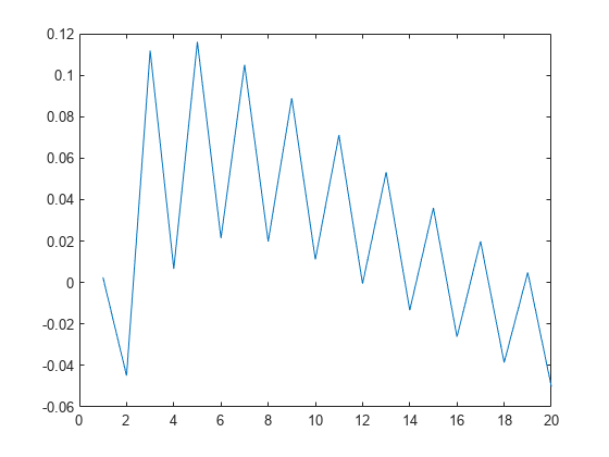
For powers of the cosine, the error oscillates between odd and even powers:

errors = zeros(1, 20);fork=1:20 errors(k) = double(sum(alpha.*(cos(x).^k)) -int(cos(t)^k*w(t), t, 0, inf));endplot(real(errors))

Figure contains an axes object. The axes object contains an object of type line.