Solve Partial Differential Equation of Nonlinear Heat Transfer

This example uses:

Open Live Script

这个例子展示了如何解决部分给出tial equation (PDE) of nonlinear heat transfer in a thin plate.

The plate is square, and its temperature is fixed along the bottom edge. No heat is transferred from the other three edges since the edges are insulated. Heat is transferred from both the top and bottom faces of the plate by convection and radiation. Because radiation is included, the problem is nonlinear.

The purpose of this example is to show how to represent the nonlinear PDE symbolically using Symbolic Math Toolbox™ and solve the PDE problem usingfinite element analysisin Partial Differential Equation Toolbox™. In this example, perform transient analysis and solve the temperature in the plate as a function of time. The transient analysis shows the time duration until the plate reaches its equilibrium temperature at steady state.

Heat Transfer Equations for the Plate

The plate has planar dimensions 1 m by 1 m and is 1 cm thick. Because the plate is relatively thin compared with the planar dimensions, the temperature can be assumed to be constant in the thickness direction, and the resulting problem is 2-D.

Assume that convection and radiation heat transfers take place between the two faces of the plate and the environment with a specified ambient temperature.

The amount of heat transferred from each plate face per unit area due to convection is defined as

$Q_{c} = h_{c} (T - T_{a})$ ,

where $T_{a}$ is the ambient temperature, $T$ is the temperature at a particular $x$ and $y$ location on the plate surface, and $h_{c}$ is a specified convection coefficient.

The amount of heat transferred from each plate face per unit area due to radiation is defined as

$Q_{r} = ϵ σ (T^{4} - T_{a}^{4})$ ,

where $ϵ$ is the emissivity of the face and $σ$ is the Stefan-Boltzmann constant. Because the heat transferred due to radiation is proportional to the fourth power of the surface temperature, the problem is nonlinear.

The PDE describing the temperature in this thin plate is

$ρ C_{p} t_{z} \frac{\partial T}{\partial t} - k t_{z} \nabla^{2} T + 2 Q_{c} + 2 Q_{r} = 0$

where $ρ$ is the material density of the plate, $C_{p}$ is its specific heat, $t_{z}$ is its plate thickness, $k$ is its thermal conductivity, and the factors of two account for the heat transfer from both of its faces.

Define PDE Parameters

Set up the PDE problem by defining the values of the parameters. The plate is composed of copper, which has the following properties.

kThermal = 400;% thermal conductivity of copper, W/(m-K)rhoCopper = 8960;% density of copper, kg/m^3specificHeat = 386;% specific heat of copper, J/(kg-K)thick = 0.01;% plate thickness in metersstefanBoltz = 5.670373e-8;% Stefan-Boltzmann constant, W/(m^2-K^4)hCoeff = 1;% convection coefficient, W/(m^2-K)tAmbient = 300;% the ambient temperatureemiss = 0.5;%板表面的发射率

Extract PDE Coefficients

Define the PDE in symbolic form with the plate temperature as a dependent variable $T (t, x, y)$ .

symsT(t,x,y)symsepssigtzhcTarhoCpkQc = hc*(T - Ta); Qr = eps*sig*(T^4 - Ta^4); pdeeq = (rho*Cp*tz*diff(T,t) - k*tz*laplacian(T,[x,y]) + 2*Qc + 2*Qr)

pdeeq(t, x, y) =
                  
                    $2 eps sig ({T (t, x, y)}^{4} - {Ta}^{4}) - k tz (\frac{\partial^{2}}{\partial x^{2}} T (t, x, y) + \frac{\partial^{2}}{\partial y^{2}} T (t, x, y)) - 2 hc (Ta - T (t, x, y)) + Cp ρ tz \frac{\partial}{\partial t} T (t, x, y)$

Now, create coefficients to use as inputs in the PDE model as required by Partial Differential Equation Toolbox. To do this, first extract the coefficients of the symbolic PDE as a structure of symbolic expressions using thepdeCoefficientsfunction.

symCoeffs = pdeCoefficients(pdeeq,T,'Symbolic',真正的)

symCoeffs =struct with fields:m: 0 a: 2*hc + 2*eps*sig*T(t, x, y)^3 c: [2x2 sym] f: 2*eps*sig*Ta^4 + 2*hc*Ta d: Cp*rho*tz

Next, substitute the symbolic variables that represent the PDE parameters with their numeric values.

symVars = [eps sig tz hc Ta rho Cp k]; symVals = [emiss stefanBoltz thick hCoeff tAmbient rhoCopper specificHeat kThermal]; symCoeffs = subs(symCoeffs,symVars,symVals);

Finally, since the fieldssymCoeffsare symbolic objects, use thepdeCoefficientsToDoublefunction to convert the coefficients to thedoubledata type, which makes them valid inputs for Partial Differential Equation Toolbox.

coeffs = pdeCoefficientsToDouble(symCoeffs)

coeffs =struct with fields:a: @makeCoefficient/coefficientFunction c: [4x1 double] m: 0 d: 3.4586e+04 f: 1.0593e+03

Specify PDE Model, Geometry, and Coefficients

Now, using Partial Differential Equation Toolbox, solve the PDE problem using finite element analysis based on these coefficients.

First, create the PDE model with a single dependent variable.

numberOfPDE = 1; model = createpde(numberOfPDE);

Specify the geometry for the PDE model—in this case, the dimension of the square.

width = 1; height = 1;

Define a geometry description matrix. Create the square geometry using thedecsg(Partial Differential Equation Toolbox)function. For a rectangular geometry, the first row contains3, and the second row contains4. The next four rows contain the $x$ -coordinates of the starting points of the edges, and the four rows after that contain the $y$ -coordinates of the starting points of the edges.

gdm = [3 4 0 width width 0 0 0 height height]'; g = decsg(gdm,'S1',('S1')');

Convert the DECSG geometry into a geometry object and include it in the PDE model.

geometryFromEdges(model,g);

Plot the geometry and display the edge labels.

figure; pdegplot(model,'EdgeLabels','on'); axis([-0.1 1.1 -0.1 1.1]); title('Geometry with Edge Labels Displayed');

Figure contains an axes object. The axes object with title Geometry with Edge Labels Displayed contains 5 objects of type line, text.

Next, create the triangular mesh in the PDE model with a mesh size of approximately 0.1 in each direction.

hmax = 0.1;% element sizemsh = generateMesh(model,'Hmax',hmax); figure; pdeplot(model); axisequaltitle('Plate with Triangular Element Mesh'); xlabel('X-coordinate, meters'); ylabel('Y-coordinate, meters');

Figure contains an axes object. The axes object with title Plate with Triangular Element Mesh contains 2 objects of type line.

Specify the coefficients in the PDE model.

specifyCoefficients(model,'m',coeffs.m,'d',coeffs.d,...'c',coeffs.c,'a',coeffs.a,'f',coeffs.f);

Find Transient Solution

Apply the boundary conditions. Three of the plate edges are insulated. Because a Neumann boundary condition equal to zero is the default in the finite element formulation, you do not need to set the boundary conditions on these edges. The bottom edge of the plate is fixed at 1000 K. Specify this using a Dirichlet condition on all nodes on the bottom edge (edge E1).

applyBoundaryCondition(model,'dirichlet',的边缘',1,'u',1000);

Specify the initial temperature to be 0 K everywhere, except at the bottom edge. Set the initial temperature on the bottom edge E1 to the value of the constant boundary condition, 1000 K.

setInitialConditions(模型中,0);setInitialConditions(model,1000,的边缘',1);

Define the time domain to find the transient solution of the PDE problem.

endTime = 10000; tlist = 0:50:endTime;

Set the tolerance of the solver options.

model.SolverOptions.RelativeTolerance = 1.0e-3; model.SolverOptions.AbsoluteTolerance = 1.0e-4;

Solve the problem usingsolvepde. Plot the temperature along the top edge of the plate as a function of time.

R = solvepde(model,tlist); u = R.NodalSolution; figure; plot(tlist,u(3,:)); gridontitle'Temperature Along the Top Edge of the Plate as a Function of Time'xlabel'Time (s)'ylabel'Temperature (K)'

Figure contains an axes object. The axes object with title Temperature Along the Top Edge of the Plate as a Function of Time contains an object of type line.

Based on the plot, the transient solution starts to reach its steady state value after 6000 seconds. The equilibrium temperature of the top edge approaches 450 K after 6000 seconds.

Show the temperature profile of the plate after 10,000 seconds.

figure; pdeplot(model,'XYData',u(:,end),'Contour','on','ColorMap','jet'); title(sprintf('Temperature in the Plate, Transient Solution (%d seconds)\n',...tlist(1,end))); xlabel'X-coordinate, meters'ylabel'Y-coordinate, meters'axisequal;

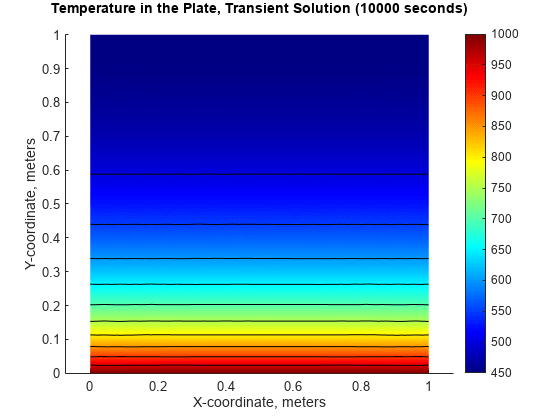
Figure contains an axes object. The axes object with title Temperature in the Plate, Transient Solution (10000 seconds) contains 12 objects of type patch, line.

Show the temperature at the top edge at 10,000 seconds.

u(3,end)

ans = 449.8031