Load Sequence Data

Load the example data.chickenpox_datasetcontains a single time series, with time steps corresponding to months and values corresponding to the number of cases. The output is a cell array, where each element is a single time step. Reshape the data to be a row vector.

data = chickenpox_dataset; data = [data{:}]; figure plot(data) xlabel("Month") ylabel("Cases") title("Monthly Cases of Chickenpox")

Partition the training and test data. Train on the first 90% of the sequence and test on the last 10%.

numTimeStepsTrain = floor(0.9*numel(data)); dataTrain = data(1:numTimeStepsTrain+1); dataTest = data(numTimeStepsTrain+1:end);

Standardize Data

For a better fit and to prevent the training from diverging, standardize the training data to have zero mean and unit variance. At prediction time, you must standardize the test data using the same parameters as the training data.

mu = mean(dataTrain); sig = std(dataTrain); dataTrainStandardized = (dataTrain - mu) / sig;

Prepare Predictors and Responses

To forecast the values of future time steps of a sequence, specify the responses to be the training sequences with values shifted by one time step. That is, at each time step of the input sequence, the LSTM network learns to predict the value of the next time step. The predictors are the training sequences without the final time step.

XTrain = dataTrainStandardized(1:end-1); YTrain = dataTrainStandardized(2:end);

Define LSTM Network Architecture

Create an LSTM regression network. Specify the LSTM layer to have 200 hidden units.

numFeatures = 1; numResponses = 1; numHiddenUnits = 200; layers = [...sequenceInputLayer(numFeatures) lstmLayer(numHiddenUnits) fullyConnectedLayer(numResponses) regressionLayer];

Specify the training options. Set the solver to'adam'and train for 250 epochs. To prevent the gradients from exploding, set the gradient threshold to 1. Specify the initial learn rate 0.005, and drop the learn rate after 125 epochs by multiplying by a factor of 0.2.

options = trainingOptions('adam',...“MaxEpochs”,250,...'GradientThreshold',1,...'InitialLearnRate',0.005,...'LearnRateSchedule','piecewise',...'LearnRateDropPeriod',125,...'LearnRateDropFactor',0.2,...'Verbose',0,...“阴谋”,'training-progress');

Train LSTM Network

Train the LSTM network with the specified training options by usingtrainNetwork.

net = trainNetwork(XTrain,YTrain,layers,options);

Forecast Future Time Steps

To forecast the values of multiple time steps in the future, use thepredictAndUpdateStatefunction to predict time steps one at a time and update the network state at each prediction. For each prediction, use the previous prediction as input to the function.

Standardize the test data using the same parameters as the training data.

dataTestStandardized = (dataTest - mu) / sig; XTest = dataTestStandardized(1:end-1);

To initialize the network state, first predict on the training dataXTrain. Next, make the first prediction using the last time step of the training responseYTrain(end). Loop over the remaining predictions and input the previous prediction topredictAndUpdateState.

For large collections of data, long sequences, or large networks, predictions on the GPU are usually faster to compute than predictions on the CPU. Otherwise, predictions on the CPU are usually faster to compute. For single time step predictions, use the CPU. To use the CPU for prediction, set the'ExecutionEnvironment'option ofpredictAndUpdateStateto'cpu'.

net = predictAndUpdateState(net,XTrain); [net,YPred] = predictAndUpdateState(net,YTrain(end)); numTimeStepsTest = numel(XTest);fori = 2:numTimeStepsTest [net,YPred(:,i)] = predictAndUpdateState(net,YPred(:,i-1),'ExecutionEnvironment','cpu');end

Unstandardize the predictions using the parameters calculated earlier.

YPred = sig*YPred + mu;

The training progress plot reports the root-mean-square error (RMSE) calculated from the standardized data. Calculate the RMSE from the unstandardized predictions.

YTest = dataTest(2:end); rmse = sqrt(mean((YPred-YTest).^2))

rmse =single248.5531

Plot the training time series with the forecasted values.

figure plot(dataTrain(1:end-1)) holdonidx = numTimeStepsTrain:(numTimeStepsTrain+numTimeStepsTest); plot(idx,[data(numTimeStepsTrain) YPred],'.-') holdoffxlabel("Month") ylabel("Cases") title("Forecast") legend(["Observed""Forecast"])

Compare the forecasted values with the test data.

figure subplot(2,1,1) plot(YTest) holdonplot(YPred,'.-') holdofflegend(["Observed""Forecast"]) ylabel("Cases") title("Forecast") subplot(2,1,2) stem(YPred - YTest) xlabel("Month") ylabel("Error") title("RMSE = "+ rmse)

Update Network State with Observed Values

如果你有访问时间的实际值eps between predictions, then you can update the network state with the observed values instead of the predicted values.

First, initialize the network state. To make predictions on a new sequence, reset the network state usingresetState. Resetting the network state prevents previous predictions from affecting the predictions on the new data. Reset the network state, and then initialize the network state by predicting on the training data.

net = resetState(net); net = predictAndUpdateState(net,XTrain);

Predict on each time step. For each prediction, predict the next time step using the observed value of the previous time step. Set the'ExecutionEnvironment'option ofpredictAndUpdateStateto'cpu'.

YPred = []; numTimeStepsTest = numel(XTest);fori = 1:numTimeStepsTest [net,YPred(:,i)] = predictAndUpdateState(net,XTest(:,i),'ExecutionEnvironment','cpu');end

Unstandardize the predictions using the parameters calculated earlier.

YPred = sig*YPred + mu;

Calculate the root-mean-square error (RMSE).

rmse = sqrt(mean((YPred-YTest).^2))

rmse = 158.0959

Compare the forecasted values with the test data.

figure subplot(2,1,1) plot(YTest) holdonplot(YPred,'.-') holdofflegend(["Observed""Predicted"]) ylabel("Cases") title("Forecast with Updates") subplot(2,1,2) stem(YPred - YTest) xlabel("Month") ylabel("Error") title("RMSE = "+ rmse)

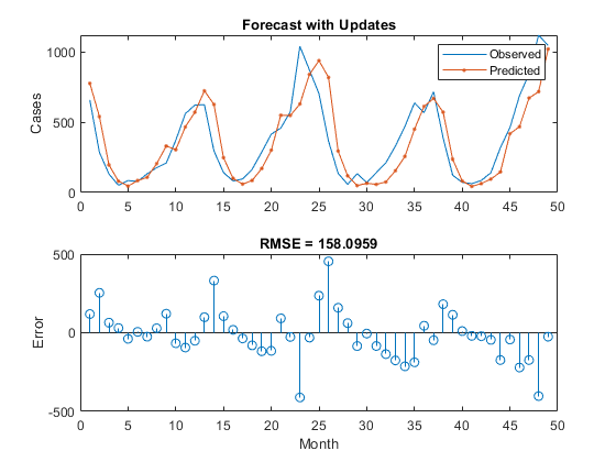
Here, the predictions are more accurate when updating the network state with the observed values instead of the predicted values.