Load Pretrained Network and Image

Load the pretrained network GoogLeNet, which will be used for image classification.

net = googlenet;

Extract the image input size and the output classes of the network.

inputSize = net.Layers(1).InputSize(1:2); classes = net.Layers(end).Classes;

Load the image. The image is of a dog named Laika. Resize the image to the network input size.

imgLaikaGrass = imread("laika_grass.jpg"); imgLaikaGrass = imresize(imgLaikaGrass,inputSize);

Classify the image, and display the three classes with the highest classification score in the image title.

[YPred,分数]=(网络,imgLai进行分类kaGrass); [~,topIdx] = maxk(scores, 3); topScores = scores(topIdx); topClasses = classes(topIdx); imshow(imgLaikaGrass) titleString = compose("%s (%.2f)",topClasses,topScores'); title(sprintf(join(titleString,"; ")));

Laika is a poodle-cocker spaniel cross. This breed is not a class in GoogLeNet, so the network has some difficulty classifying the image. The network is not very confident in its predictions — the predicted classminiature poodleonly has a score of 23%. The class with the next highest score is also a type of poodle, which is a reasonable classification. The network also assigns a moderate probability to theTibetan terrierclass. We can use occlusion to understand which parts of the image cause the network to suggest these three classes.

Identify Areas of an Image the Network Uses for Classification

You can use occlusion to find out which parts of the image are important for the classification. First, look at the predicted class ofminiature poodle. What parts of the image suggest this class? Use the occlusion sensitivity function to map the change in the classification score when parts of the image are occluded.

map = occlusionSensitivity(net,imgLaikaGrass,YPred);

Display the image of Laika with the occlusion sensitivity map overlaid.

imshow (imgLaikaGrass'InitialMagnification', 150) holdonimagesc(map,'AlphaData',0.5) colormapjetcolorbar title(sprintf("Occlusion sensitivity (%s)",...YPred))

The occlusion map shows which parts of the image have a positive contribution to the score for theminiature poodleclass, and which parts have a negative contribution. Red areas of the map have a higher value and are evidence for theminiature poodleclass — when the red areas are obscured, the score forminiature poodlegoes down. In this image, Laika's head, back, and ears provide the strongest evidence for theminiature poodleclass.

Blue areas of the map with lower values are parts of the image that lead to an increase in the score forminiature poodle当堵塞。通常,这些areas are evidence of another class, and can confuse the network. In this case, Laika's mouth and legs have a negative contribution to the overall score forminiature poodle.

The occlusion map is strongly focused on the dog in the image, which shows that GoogLeNet is classifying the correct object in the image. If your network is not producing the results you expect, an occlusion map can help you understand why. For example, if the network is strongly focused on other parts of the image, this suggests that the network learned the wrong features.

You can get similar results using the gradient class activation mapping (Grad-CAM) technique. Grad-CAM uses the gradient of the classification score with respect to the last convolutional layer in a network in order to understand which parts of the image are most important for classification. For an example, seeGrad-CAM Reveals the Why Behind Deep Learning Decisions.

Occlusion sensitivity and Grad-CAM usually return qualitatively similar results, although they work in different ways. Typically, you can compute the Grad-CAM map faster that the occlusion map, without tuning any parameters. However, the Grad-CAM map can usually has a lower spatial resolution than an occlusion map and can miss fine details. The underlying resolution of Grad-CAM is the spatial resolution of the last convolutional feature map; in the case of GoogleNet this is 7-by-7 pixels. To get the best results from occlusion sensitivity, you must choose the right values for theMaskSizeandStrideoptions. This tuning provides more flexibility to examine the input features at different length scales.

Compare Evidence for Different Classes

You can use occlusion to compare which parts of the image the network identifies as evidence for different classes. This can be useful in cases where the network is not confident in the classification and gives similar scores to several classes.

Compute an occlusion map for each of the top three classes. To examine the results of occlusion with higher resolution, reduce the mask size and stride using theMaskSizeandStrideoptions. A smallerStrideleads to a higher-resolution map, but can take longer to compute and use more memory. A smallerMaskSizeillustrates smaller details, but can lead to noisier results.

topClasses = classes(topIdx); topClassesMap = occlusionSensitivity(net, imgLaikaGrass, topClasses,..."Stride", 10,..."MaskSize", 15);

Plot the results for each of the top three classes.

fori=1:length(topIdx) figure imshow(imgLaikaGrass); holdonimagesc(topClassesMap(:,:,i),'AlphaData', 0.5); colormapjet; classLabel = string(classes(topIdx(i))); title(sprintf("%s", classLabel));end

Different parts of the image have a very different impact on the class scores for different dog breeds. The dog's back has a strong influence in favor of theminiature poodleandtoy poodleclasses, while the mouth and ears contribute to theTibetan terrierclass.

Investigate Misclassification Issues

If your network is consistently misclassifying certain types of input data, you can use occlusion sensitivity to determine if particular features of your input data are confusing the network. From the occlusion map of Laika sitting on the grass, you could expect that images of Laika which are more focused on her face are likely to be misclassified asTibetan terrier. You can verify that this is the case using another image of Laika.

imgLaikaSit = imresize(imread("laika_sitting.jpg"), inputSize);[YPred,分数]=(网络,imgLai进行分类kaSit); [score,idx] = max(scores); YPred, score

YPred =categoricalTibetan terrier

score =single0.5668

Compute the occlusion map of the new image.

map = occlusionSensitivity(net,imgLaikaSit,YPred); imshow(imgLaikaSit); holdon; imagesc(map,'AlphaData', 0.5); colormapjet; title(sprintf("%s (%.2f)",...string(classes(idx)),score));

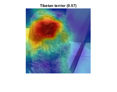
Again, the network strongly associates the dog's nose and mouth with theTibetan terrierclass. This highlights a possible failure mode of the network, since it suggests that images of Laika's face will consistently be misclassified asTibetan terrier.

You can use the insights gained from theocclusionSensitivityfunction to make sure your network is focusing on the correct features of the input data. The cause of the classification problem in this example is that the available classes of GoogleNet do not include cross-breed dogs like Laika. The occlusion map demonstrates why the network is confused by these images of Laika. It is important to be sure that the network you are using is suitable for the task at hand.

在这个例子中,网络是错误地identifying different parts of the object in the image as different classes. One solution to this issue is to retrain the network with more labeled data that covers a wider range of observations of the misclassified class. For example, the network here could be retrained using a large number of images of Laika taken at different angles, so that it learns to associate both the back and the front of the dog with the correct class.

References

[1] Zeiler M.D., Fergus R. (2014) Visualizing and Understanding Convolutional Networks. In: Fleet D., Pajdla T., Schiele B., Tuytelaars T. (eds) Computer Vision – ECCV 2014. ECCV 2014. Lecture Notes in Computer Science, vol 8689. Springer, Cham