Train Network Using Custom Training Loop

Open Live Script

This example shows how to train a network that classifies handwritten digits with a custom learning rate schedule.

You can train most types of neural networks using thetrainNetworkandtrainingOptionsfunctions. If thetrainingOptionsfunction does not provide the options you need (for example, a custom learning rate schedule), then you can define your own custom training loop usingdlarrayanddlnetworkobjects for automatic differentiation. For an example showing how to retrain a pretrained deep learning network using thetrainNetworkfunction, seeTransfer Learning Using Pretrained Network.

Training a deep neural network is an optimization task. By considering a neural network as a function $f (X; θ)$ , where $X$ is the network input, and $θ$ is the set of learnable parameters, you can optimize $θ$ so that it minimizes some loss value based on the training data. For example, optimize the learnable parameters $θ$ such that for a given inputs $X$ with a corresponding targets $T$ , they minimize the error between the predictions $Y = f (X; θ)$ and $T$ .

取决于使用的损失函数类型的任务. For example:

For classification tasks, you can minimize the cross entropy error between the predictions and targets.
For regression tasks, you can minimize the mean squared error between the predictions and targets.

You can optimize the objective using gradient descent: minimize the loss $L$ by iteratively updating the learnable parameters $θ$ by taking steps towards the minimum using the gradients of the loss with respect to the learnable parameters. Gradient descent algorithms typically update the learnable parameters by using a variant of an update step of the form $θ_{t + 1} = θ_{t} - ρ \nabla L$ , where $t$ is the iteration number, $ρ$ is the learning rate, and $\nabla L$ denotes the gradients (the derivatives of the loss with respect to the learnable parameters).

This example trains a network to classify handwritten digits with thetime-based decaylearning rate schedule: for each iteration, the solver uses the learning rate given by $ρ_{t} = \frac{ρ_{0}}{1 + k t}$ , wheretis the iteration number, $ρ_{0}$ is the initial learning rate, andkis the decay.

Load Training Data

Load the digits data as an image datastore using theimageDatastorefunction and specify the folder containing the image data.

dataFolder = fullfile(toolboxdir("nnet"),"nndemos","nndatasets","DigitDataset"); imds = imageDatastore(dataFolder,...IncludeSubfolders=true,....LabelSource="foldernames");

Partition the data into training and validation sets. Set aside 10% of the data for validation using thesplitEachLabelfunction.

[imdsTrain,imdsValidation] = splitEachLabel(imds,0.9,"randomize");

The network used in this example requires input images of size 28-by-28-by-1. To automatically resize the training images, use an augmented image datastore. Specify additional augmentation operations to perform on the training images: randomly translate the images up to 5 pixels in the horizontal and vertical axes. Data augmentation helps prevent the network from overfitting and memorizing the exact details of the training images.

inputSize = [28 28 1]; pixelRange = [-5 5]; imageAugmenter = imageDataAugmenter(...RandXTranslation=pixelRange,...RandYTranslation=pixelRange); augimdsTrain = augmentedImageDatastore(inputSize(1:2),imdsTrain,DataAugmentation=imageAugmenter);

To automatically resize the validation images without performing further data augmentation, use an augmented image datastore without specifying any additional preprocessing operations.

augimdsValidation = augmentedImageDatastore(inputSize(1:2),imdsValidation);

Determine the number of classes in the training data.

classes = categories(imdsTrain.Labels); numClasses = numel(classes);

Define Network

Define the network for image classification.

For image input, specify an image input layer with input size matching the training data.
Do not normalize the image input, set theNormalizationoption of the input layer to"none".
Specify three convolution-batchnorm-ReLU blocks.
Pad the input to the convolution layers such that the output has the same size by setting thePaddingoption to"same".
For the first convolution layer specify 20 filters of size 5. For the remaining convolution layers specify 20 filters of size 3.
For classification, specify a fully connected layer with size matching the number of classes
To map the output to probabilities, include a softmax layer.

When training a network using a custom training loop, do not include an output layer.

layers = [ imageInputLayer(inputSize,Normalization="none") convolution2dLayer(5,20,Padding="same") batchNormalizationLayer reluLayer convolution2dLayer(3,20,Padding="same") batchNormalizationLayer reluLayer convolution2dLayer(3,20,Padding="same") batchNormalizationLayer reluLayer fullyConnectedLayer(numClasses) softmaxLayer];

Create adlnetworkobject from the layer array.

net = dlnetwork(layers)

net = dlnetwork with properties: Layers: [12×1 nnet.cnn.layer.Layer] Connections: [11×2 table] Learnables: [14×3 table] State: [6×3 table] InputNames: {'imageinput'} OutputNames: {'softmax'} Initialized: 1

Define Model Loss Function

Create the functionmodelLoss, listed in theModel Loss Functionsection of the example, that takes as input thedlnetworkobject, a mini-batch of input data with corresponding targets, and returns the loss, the gradients of the loss with respect to the learnable parameters, and the network state.

Specify Training Options

Train for ten epochs with a mini-batch size of 128.

numEpochs = 10; miniBatchSize = 128;

Specify the options for SGDM optimization. Specify an initial learn rate of 0.01 with a decay of 0.01, and momentum 0.9.

initialLearnRate = 0.01; decay = 0.01; momentum = 0.9;

Train Model

Create aminibatchqueueobject that processes and manages mini-batches of images during training. For each mini-batch:

Use the custom mini-batch preprocessing functionpreprocessMiniBatch(defined at the end of this example) to convert the labels to one-hot encoded variables.
Format the image data with the dimension labels"SSCB"(spatial, spatial, channel, batch). By default, theminibatchqueueobject converts the data todlarrayobjects with underlying typesingle. Do not format the class labels.
Train on a GPU if one is available. By default, theminibatchqueueobject converts each output to agpuArrayif a GPU is available. Using a GPU requires Parallel Computing Toolbox™ and a supported GPU device. For information on supported devices, seeGPU Support by Release(Parallel Computing Toolbox).

mbq = minibatchqueue(augimdsTrain,...MiniBatchSize=miniBatchSize,...MiniBatchFcn=@preprocessMiniBatch,...MiniBatchFormat=["SSCB"""]);

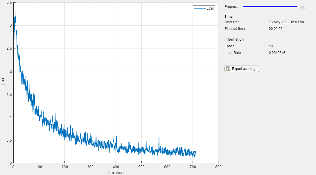
Initialize the training progress plot.

figure C = colororder; lineLossTrain = animatedline(Color=C(2,:)); ylim([0 inf]) xlabel("Iteration") ylabel("Loss") gridon

Initialize the velocity parameter for the SGDM solver.

velocity = [];

Train the network using a custom training loop. For each epoch, shuffle the data and loop over mini-batches of data. For each mini-batch:

Evaluate the model loss, gradients, and state using thedlfevalandmodelLossfunctions and update the network state.
Determine the learning rate for the time-based decay learning rate schedule.
Update the network parameters using thesgdmupdatefunction.
Display the training progress.

iteration = 0; start = tic;% Loop over epochs.forepoch = 1:numEpochs% Shuffle data.shuffle(mbq);% Loop over mini-batches.whilehasdata(mbq) iteration = iteration + 1;% Read mini-batch of data.[X,T] = next(mbq);% Evaluate the model gradients, state, and loss using dlfeval and the% modelLoss function and update the network state.[loss,gradients,state] = dlfeval(@modelLoss,net,X,T); net.State = state;% Determine learning rate for time-based decay learning rate schedule.learnRate = initialLearnRate/(1 + decay*iteration);% Update the network parameters using the SGDM optimizer.[net,velocity] = sgdmupdate(net,gradients,velocity,learnRate,momentum);% Display the training progress.D = duration(0,0,toc(start),Format="hh:mm:ss"); loss = double(loss); addpoints(lineLossTrain,iteration,loss) title("Epoch: "+ epoch +", Elapsed: "+ string(D)) drawnowendend

Test Model

Test the classification accuracy of the model by comparing the predictions on the validation set with the true labels.

After training, making predictions on new data does not require the labels. Createminibatchqueueobject containing only the predictors of the test data:

To ignore the labels for testing, set the number of outputs of the mini-batch queue to 1.
Specify the same mini-batch size used for training.
Preprocess the predictors using thepreprocessMiniBatchPredictorsfunction, listed at the end of the example.
For the single output of the datastore, specify the mini-batch format"SSCB"(spatial, spatial, channel, batch).

numOutputs = 1; mbqTest = minibatchqueue(augimdsValidation,numOutputs,...MiniBatchSize=miniBatchSize,...MiniBatchFcn = @preprocessMiniBatchPredictors,...MiniBatchFormat="SSCB");

Loop over the mini-batches and classify the images usingmodelPredictionsfunction, listed at the end of the example.

YTest = modelPredictions(net,mbqTest,classes);

Evaluate the classification accuracy.

TTest = imdsValidation.Labels; accuracy = mean(TTest == YTest)

accuracy = 0.7210

Visualize the predictions in a confusion chart.

figure confusionchart(TTest,YTest)

Large values on the diagonal indicate accurate predictions for the corresponding class. Large values on the off-diagonal indicate strong confusion between the corresponding classes.

Supporting Functions

Model Loss Function

ThemodelLossfunction takes adlnetworkobjectnet, a mini-batch of input dataXwith corresponding targetsTand returns the loss, the gradients of the loss with respect to the learnable parameters innet, and the network state. To compute the gradients automatically, use thedlgradientfunction.

function[loss,gradients,state] = modelLoss(net,X,T)% Forward data through network.[Y,state] = forward(net,X);% Calculate cross-entropy loss.loss = crossentropy(Y,T);% Calculate gradients of loss with respect to learnable parameters.gradients = dlgradient(loss,net.Learnables);end

Model Predictions Function

ThemodelPredictionsfunction takes adlnetworkobjectnet, aminibatchqueueof input datambq, and the network classes, and computes the model predictions by iterating over all data in theminibatchqueueobject. The function uses theonehotdecodefunction to find the predicted class with the highest score.

functionY = modelPredictions(net,mbq,classes) Y = [];% Loop over mini-batches.whilehasdata(mbq) X = next(mbq);% Make prediction.scores = predict(net,X);% Decode labels and append to output.labels = onehotdecode(scores,classes,1)'; Y = [Y; labels];endend

Mini Batch Preprocessing Function

ThepreprocessMiniBatchfunction preprocesses a mini-batch of predictors and labels using the following steps:

Preprocess the images using thepreprocessMiniBatchPredictorsfunction.
从传入细胞arra提取标签数据y and concatenate into a categorical array along the second dimension.
One-hot encode the categorical labels into numeric arrays. Encoding into the first dimension produces an encoded array that matches the shape of the network output.

function[X,T] = preprocessMiniBatch(dataX,dataT)% Preprocess predictors.X = preprocessMiniBatchPredictors(dataX);% Extract label data from cell and concatenate.T = cat(2,dataT{1:end});% One-hot encode labels.T = onehotencode(T,1);end

Mini-Batch Predictors Preprocessing Function

ThepreprocessMiniBatchPredictorsfunction preprocesses a mini-batch of predictors by extracting the image data from the input cell array and concatenate into a numeric array. For grayscale input, concatenating over the fourth dimension adds a third dimension to each image, to use as a singleton channel dimension.

functionX = preprocessMiniBatchPredictors(dataX)% Concatenate.X = cat(4,dataX{1:end});end