数据和拟合模型

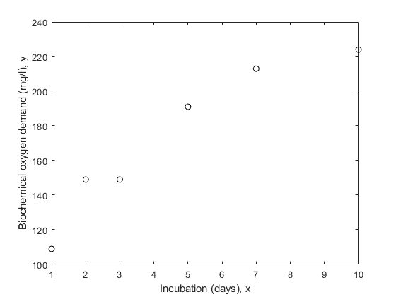
We'll use data collected to study water pollution caused by industrial and domestic waste. These data are described in detail in Box, G.P., W.G. Hunter, and J.S. Hunter, Statistics for Experimenters (Wiley, 1978, pp. 483-487). The response variable is biochemical oxygen demand in mg/l, and the predictor variable is incubation time in days.

x = [1 2 3 5 7 10]';y = [109 149 149 191 213 224]';情节（x，y，'ko'）xlabel('Incubation (days), x'）ylabel('Biochemical oxygen demand (mg/l), y'）

我们假设已知前两个观察结果的精度低于其余观察结果。例如，它们可能是用不同的工具制成的。加权数据的另一个常见原因是，每个记录的观察结果实际上是以x相同值进行的几个测量值的平均值。在此处的数据中，假设前两个值代表单个原始测量值，而其余四个值则是5个原始测量值的平均值。然后，通过进入每个观察结果的测量数量来加重。

w = [1 1 5 5 5 5]';

Fit the Model without Weights

我们将适合这些数据的模型是一个缩放的指数曲线，随着X变大，该曲线变为水平。

modelFun = @(b,x) b(1).*(1-exp(-b(2).*x));

仅基于粗糙的视觉拟合，看来通过点绘制的曲线可能会在X = 15附近的某个地方的240个值中升级。因此，我们将使用240作为B1的起始值，并且由于e^（ - 。5*15）与1相比小，我们将.5用作B2的起始值。

开始= [240;.5];

这danger in ignoring measurement error is that the fit may be overly influenced by imprecise measurements, and may therefore not provide a good fit to measurements that are known precisely. Let's fit the data without weights and compare it to the points.

nlm = fitnlm(x,y,modelFun,start); xx = linspace(0,12)'; line(xx,predict(nlm,xx),'linestyle'，，，，'--'，，，，'颜色'，，，，'k'）

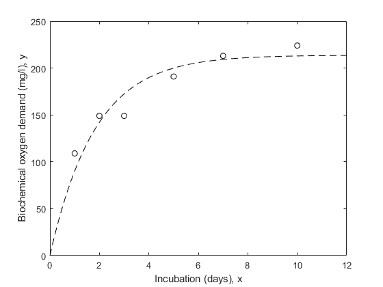
Notice that the fitted curve is pulled toward the first two points, but seems to miss the trend of the other points.

用重量安装模型

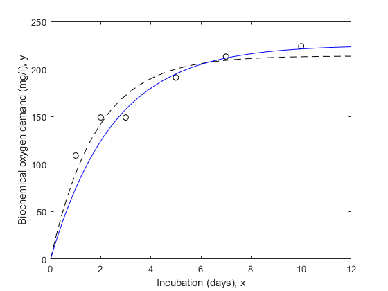
Let's try repeating the fit using weights.

wnlm = fitnlm（x，y，modelfun，start，'Weight'，，，，w)

wnlm = Nonlinear regression model: y ~ b1*(1 - exp( - b2*x)) Estimated Coefficients: Estimate SE tStat pValue ________ ________ ______ __________ b1 225.17 10.7 21.045 3.0134e-05 b2 0.40078 0.064296 6.2333 0.0033745 Number of observations: 6，误差自由度：4根平方误差：24 R平方：0.908，调整后的R平方0.885 F统计与零模型：696，p-value = 8.2e-06

线（xx，预测（wnlm，xx），'颜色'，，，，'b'）

在这种情况下，估计的种群标准偏差描述了重量或测量精度为1的“标准”观察的平均差异。

wnlm.RMSE

ANS = 24.0096

任何分析的重要部分是估计模型拟合的精度。系数显示显示参数的标准错误，但我们还可以为其计算置信区间。

COEFCI(wnlm)

ans =2×2195.4650 254.8788 0.2223 0.5793

Estimate the Response Curve

Next, we'll compute the fitted response values and confidence intervals for them. By default, those widths are for pointwise confidence bounds for the predicted value, but we will request simultaneous intervals for the entire curve.

[ypred,ypredci] = predict(wnlm,xx,'Simultaneous'，真的）;情节（x，y，'ko'，xx，ypred，'b-'，，，，xx,ypredci,'r:'）xlabel('x'）ylabel('y'）ylim([-150 350]) legend({'Data'，，，，'Weighted fit'，，，，'95% Confidence Limits'},...'location'，，，，'SouthEast'）

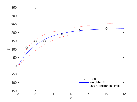
Notice that the two downweighted points are not fit as well by the curve as the remaining points. That's as you would expect for a weighted fit.

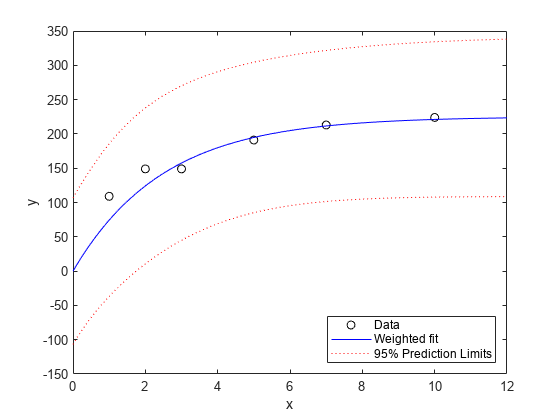
It's also possible to estimate prediction intervals for future observations at specified values of x. Those intervals will in effect assume a weight, or measurement precision, of 1.

[ypred,ypredci] = predict(wnlm,xx,'Simultaneous'，真的，...'Prediction'，，，，'observation'）; plot(x,y,'ko'，xx，ypred，'b-'，，，，xx,ypredci,'r:'）xlabel('x'）ylabel('y'）ylim([-150 350]) legend({'Data'，，，，'Weighted fit'，，，，'95％的预测限制'},...'location'，，，，'SouthEast'）

权重的绝对尺度实际上不会影响参数估计。将权重缩放任何常数都会给我们相同的估计。但是它们确实会影响置信度界限，因为边界代表了重量1的观察。在这里，您可以看到，与置信度限制相比，重量更高的点似乎太接近了拟合线路。

Suppose we are interested in a new observation that is based on the average of five measurements, just like the last four points in this plot. Specify observation weights by using the权重name-value argument of thepredictfunction.

[new_ypred,new_ypredci] = predict(wnlm,xx,'Simultaneous'，真的，...'Prediction'，，，，'observation'，，，，“重量”，，，，5*ones(size(xx))); plot(x,y,'ko'，，，，xx,new_ypred,'b-'，，，，xx,new_ypredci,'r:'）xlabel('x'）ylabel('y'）ylim([-150 350]) legend({'Data'，，，，'Weighted fit'，，，，'95％的预测限制'},...'location'，，，，'SouthEast'）

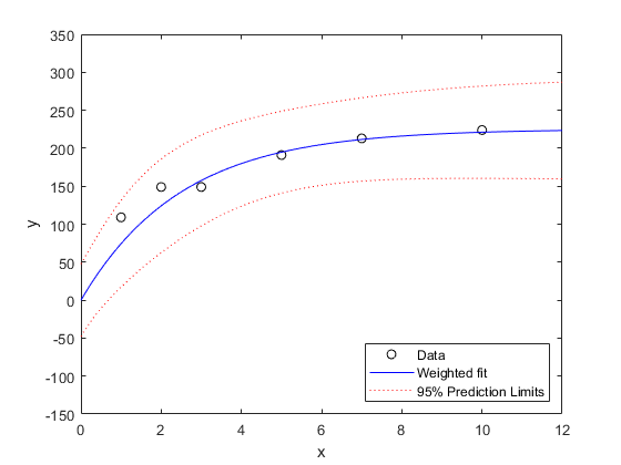
这predictfunction estimates the error variance at observation一世经过MSE*(1/W(i))，，，，whereMSE一世s the mean squared error. Therefore, the confidence intervals become narrow.

剩余分析

除了绘制数据和拟合度之外，还将残差从与预测变量相对的拟合中绘制，以诊断模型的任何问题。残差应显得独立且分布相同（i.i.d。），但与权重倒数成正比。绘制标准化残差，以确认值是I.I.D.具有相同的差异。标准化残差是原始残留物除以其估计的标准偏差。

r = wnlm.Residuals.Standardized; plot(x,r,'b^'）xlabel('x'）ylabel('Standardized Residuals'）

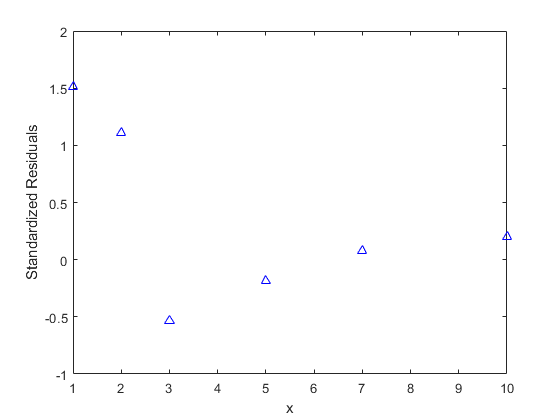
在此残差图中有一些系统模式的证据。请注意，最后四个残差是如何具有线性趋势的，表明该模型随着X的增加可能不够快。同样，随着X的增加，残差的大小往往会减小，这表明测量误差可能取决于x。但是，这些值得研究的数据点很少，因此很难对这些明显模式具有重要意义。