Getting Started with RF Modeling

This example uses:

Open Script

Learn how to use theRF Budget Analyzerapp to build a simple RF receiver, and then create an RF Blockset™ Circuit Envelope multi-carrier model to perform simulation.

Build a Cascade (row vector) of RF Elements.

You can build and analyze an RF cascade by adding elements characterized by their data sheet specifications.

You can use theRF Budget Analyserapp and drag and drop new elements, or you can script the chain elements using MATLAB® commands. If you are not familiar with the syntax, you can start with app and generate a MATLAB script.

Add elements to your chain in the following order:

Filter specified by an S-parameters Touchstone file
Low Noise Amplifier (LNA)
Direct conversion demodulator
Baseband amplifier

elements(1) = nport('sawfilterpassive.s2p'); elements(2) = amplifier(...'Name','LNA',...“获得”,18,...'NF',3,...'OIP3',10); elements(3) = modulator(...'Name','Demod',...“获得”,10,...'NF',6.4,...'OIP3',36,...'LO',2.45e9,...'ConverterType','Down'); elements(4) = amplifier(...“获得”,20,...'NF',11.3,...'OIP3',42);

Inspect RF Budget Using RF Budget Analyzer App

Create anrfbudgetobject. The MATLAB command window dynamically displays the budget analysis results.

b = rfbudget(...'Elements',elements,...'InputFrequency',2.45e9,...'AvailableInputPower',-70,...'SignalBandwidth',8e6)

b = rfbudget with properties: Elements: [1x4 rf.internal.rfbudget.Element] InputFrequency: 2.45 GHz AvailableInputPower: -70 dBm SignalBandwidth: 8 MHz Solver: Friis AutoUpdate: true Analysis Results OutputFrequency: (GHz) [ 2.45 2.45 0 0] OutputPower: (dBm) [-73.04 -55.04 -45.04 -25.04] TransducerGain: (dB) [-3.044 14.96 24.96 44.96] NF: (dB) [ 2.326 5.699 5.823 5.868] IIP2: (dBm) [] OIP2: (dBm) [] IIP3: (dBm) [ Inf -5.674 -5.782 -7.865] OIP3: (dBm) [ Inf 10 19.89 37.81] SNR: (dB) [ 32.62 29.25 29.12 29.08]

Or you can visualize therfbudgetobject in the app using the MATLAB commandshow(b).

Generate RF Blockset Model

Use theExportbutton in theRF Budget Analyzerapp to create an RF Blockset model or:

exportRFBlockset(b) save_system(gcs,'model_1')

You can use this model for multi-carrier circuit envelope simulation. TheInput Port/Output Portports and配置block are set up correctly and you can copy the model for use in any other Simulink® testbench.

The input port specifies a complex powerwave signal centered at 2.45 GHz.
The output ports terminate the cascade and extract the envelope centered at DC (0 Hz). The I and Q signals are real baseband signals.
The Configuration block runs the simulation for a total of 8 simulation frequencies in order to capture the non linearity introduced by the demodulator and amplifiers.
The simulation stop time in this case is set equal to 0. This means that the simulation does only a static analysis of the model (harmonic balance).

Observe and understand the model blocks:

The S-parameter block describing the filter uses rational fitting in order to simulate frequency data in the time domain. Notice that at 2.45 GHz it introduces a phase rotation of approximately -58 degrees.
Both amplifiers specify IP3, but you can also specify IP2.
The demodulator includes ideal channel selection filters. Additional impairments can be added such as LO leakage and I/Q imbalance.

Simulate the model to compare the output power values with theRF Budget Analyzerapp values. Notice that due to the phase rotation introduced by the S-parameter block, the complex input signal is partly downconverted on the I and on the Q branch, and thus the output power on the two branches is different. For this reason, the gain and other specs of direct conversion receivers, are measured at an arbitrary low frequency.

生成我asurement Testbench

Use theExportbutton in theRF Budget Analyzerapp to create a measurement testbench or:

exportTestbench(b) save_system(gcs,'model_2')

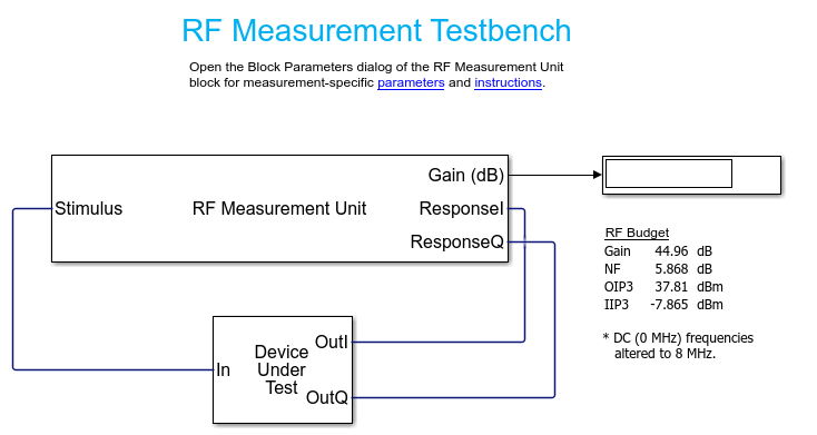
To measure the gain, noise figure, and OIP3 use the RF Measurement Unit dialog box to choose the value you want to verify.

Observe and understand the testbench block:

You can measure the output on the I or Q branches.
Measurements are done at an arbitrary low frequency
Measurements are done in the time domain over an arbitrary signal bandwidth

Run the following simulation:

Measure the gain (disable the noise for accurate measurements).
Measure the NF. Reduce the baseband bandwidth to 8e3 for narrowband measurements. In this way, the noise figure measurement is not affected by the filter selectivity.
Measure the OIP3. Keep the smaller baseband bandwidth and disable noise for accurate measurements.

On comparing, you will see that the values of gain, noise figure, and IP3 match the values in theRF Budget Analyzerapp reported in the testbench.

Getting Started with RF Modeling

Build a Cascade (row vector) of RF Elements.

Inspect RF Budget Using RF Budget Analyzer App

Generate RF Blockset Model

生成我asurement Testbench

See Also

RF Blockset Documentation

金宝app

Try MATLAB, Simulink, and Other Products