IMU and GPS Fusion for Inertial Navigation

Open Live Script

This example shows how you might build an IMU + GPS fusion algorithm suitable for unmanned aerial vehicles (UAVs) or quadcopters.

This example uses accelerometers, gyroscopes, magnetometers, and GPS to determine orientation and position of a UAV.

Simulation Setup

Set the sampling rates. In a typical system, the accelerometer and gyroscope run at relatively high sample rates. The complexity of processing data from those sensors in the fusion algorithm is relatively low. Conversely, the GPS, and in some cases the magnetometer, run at relatively low sample rates, and the complexity associated with processing them is high. In this fusion algorithm, the magnetometer and GPS samples are processed together at the same low rate, and the accelerometer and gyroscope samples are processed together at the same high rate.

To simulate this configuration, the IMU (accelerometer, gyroscope, and magnetometer) are sampled at 160 Hz, and the GPS is sampled at 1 Hz. Only one out of every 160 samples of the magnetometer is given to the fusion algorithm, so in a real system the magnetometer could be sampled at a much lower rate.

imuFs = 160; gpsFs = 1;% Define where on the Earth this simulated scenario takes place using the% latitude, longitude and altitude.refloc = [42.2825 -72.3430 53.0352];% Validate that the |gpsFs| divides |imuFs|. This allows the sensor sample% rates to be simulated using a nested for loop without complex sample rate% matching.imuSamplesPerGPS = (imuFs/gpsFs); assert(imuSamplesPerGPS == fix(imuSamplesPerGPS),...'GPS sampling rate must be an integer factor of IMU sampling rate.');

Fusion Filter

Create the filter to fuse IMU + GPS measurements. The fusion filter uses an extended Kalman filter to track orientation (as a quaternion), velocity, position, sensor biases, and the geomagnetic vector.

ThisinsfilterMARGhas a few methods to process sensor data, includingpredict,fusemagandfusegps. Thepredictmethod takes the accelerometer and gyroscope samples from the IMU as inputs. Call thepredictmethod each time the accelerometer and gyroscope are sampled. This method predicts the states one time step ahead based on the accelerometer and gyroscope. The error covariance of the extended Kalman filter is updated here.

Thefusegpsmethod takes GPS samples as input. This method updates the filter states based on GPS samples by computing a Kalman gain that weights the various sensor inputs according to their uncertainty. An error covariance is also updated here, this time using the Kalman gain as well.

Thefusemagmethod is similar but updates the states, Kalman gain, and error covariance based on the magnetometer samples.

Though theinsfilterMARGtakes accelerometer and gyroscope samples as inputs, these are integrated to compute delta velocities and delta angles, respectively. The filter tracks the bias of the magnetometer and these integrated signals.

fusionfilt = insfilterMARG; fusionfilt.IMUSampleRate = imuFs; fusionfilt.ReferenceLocation = refloc;

UAV Trajectory

This example uses a saved trajectory recorded from a UAV as the ground truth. This trajectory is fed to several sensor simulators to compute simulated accelerometer, gyroscope, magnetometer, and GPS data streams.

% Load the "ground truth" UAV trajectory.loadLoggedQuadcopter.mattrajData; trajOrient = trajData.Orientation; trajVel = trajData.Velocity; trajPos = trajData.Position; trajAcc = trajData.Acceleration; trajAngVel = trajData.AngularVelocity;% Initialize the random number generator used in the simulation of sensor% noise.rng(1)

GPS Sensor

Set up the GPS at the specified sample rate and reference location. The other parameters control the nature of the noise in the output signal.

gps = gpsSensor('UpdateRate', gpsFs);gps。ReferenceLocation = refloc;gps。十yFactor = 0.5;% Random walk noise parametergps。HorizontalPositionAccuracy = 1.6; gps.VerticalPositionAccuracy = 1.6; gps.VelocityAccuracy = 0.1;

IMU Sensors

Typically, a UAV uses an integrated MARG sensor (Magnetic, Angular Rate, Gravity) for pose estimation. To model a MARG sensor, define an IMU sensor model containing an accelerometer, gyroscope, and magnetometer. In a real-world application the three sensors could come from a single integrated circuit or separate ones. The property values set here are typical for low-cost MEMS sensors.

imu = imuSensor('accel-gyro-mag','SampleRate', imuFs); imu.MagneticField = [19.5281 -5.0741 48.0067];% Accelerometerimu.Accelerometer.MeasurementRange = 19.6133; imu.Accelerometer.Resolution = 0.0023928; imu.Accelerometer.ConstantBias = 0.19; imu.Accelerometer.NoiseDensity = 0.0012356;% Gyroscopeimu.Gyroscope.MeasurementRange = deg2rad(250); imu.Gyroscope.Resolution = deg2rad(0.0625); imu.Gyroscope.ConstantBias = deg2rad(3.125); imu.Gyroscope.AxesMisalignment = 1.5; imu.Gyroscope.NoiseDensity = deg2rad(0.025);% Magnetometerimu.Magnetometer.MeasurementRange = 1000; imu.Magnetometer.Resolution = 0.1; imu.Magnetometer.ConstantBias = 100; imu.Magnetometer.NoiseDensity = 0.3/ sqrt(50);

Initialize the State Vector of the`insfilterMARG`

TheinsfilterMARGtracks the pose states in a 22-element vector. The states are:

State Units State Vector Index Orientation as a quaternion 1:4 Position (NED) m 5:7 Velocity (NED) m/s 8:10 Delta Angle Bias (XYZ) rad 11:13 Delta Velocity Bias (XYZ) m/s 14:16 Geomagnetic Field Vector (NED) uT 17:19 Magnetometer Bias (XYZ) uT 20:22

Ground truth is used to help initialize the filter states, so the filter converges to good answers quickly.

% Initialize the states of the filterinitstate = zeros(22,1); initstate(1:4) = compact( meanrot(trajOrient(1:100))); initstate(5:7) = mean( trajPos(1:100,:), 1); initstate(8:10) = mean( trajVel(1:100,:), 1); initstate(11:13) = imu.Gyroscope.ConstantBias./imuFs; initstate(14:16) = imu.Accelerometer.ConstantBias./imuFs; initstate(17:19) = imu.MagneticField; initstate(20:22) = imu.Magnetometer.ConstantBias; fusionfilt.State = initstate;

Initialize the Variances of the`insfilterMARG`

TheinsfilterMARGmeasurement noises describe how much noise is corrupting the sensor reading. These values are based on theimuSensorandgpsSensorparameters.

The process noises describe how well the filter equations describe the state evolution. Process noises are determined empirically using parameter sweeping to jointly optimize position and orientation estimates from the filter.

% Measurement noisesRmag = 0.0862;% Magnetometer measurement noiseRvel = 0.0051;% GPS Velocity measurement noiseRpos = 5.169;% GPS Position measurement noise% Process noisesfusionfilt.AccelerometerBiasNoise = 0.010716; fusionfilt.AccelerometerNoise = 9.7785; fusionfilt.GyroscopeBiasNoise = 1.3436e-14; fusionfilt.GyroscopeNoise = 0.00016528; fusionfilt.MagnetometerBiasNoise = 2.189e-11; fusionfilt.GeomagneticVectorNoise = 7.67e-13;% Initial error covariancefusionfilt.StateCovariance = 1e-9*eye(22);

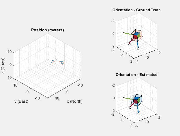
Initialize Scopes

TheHelperScrollingPlotterscope enables plotting of variables over time. It is used here to track errors in pose. TheHelperPoseViewerscope allows 3-D visualization of the filter estimate and ground truth pose. The scopes can slow the simulation. To disable a scope, set the corresponding logical variable tofalse.

useErrScope = true;% Turn on the streaming error plotusePoseView = true;% Turn on the 3-D pose viewerifuseErrScope errscope = HelperScrollingPlotter(...'NumInputs', 4,...'TimeSpan', 10,...'SampleRate', imuFs,...'YLabel', {'degrees',...'meters',...'meters',...'meters'},...'Title', {'Quaternion Distance',...'Position X Error',...“Y位置错误”,...'Position Z Error'},...'YLimits',...[ -3, 3 -2, 2 -2 2 -2 2]);endifusePoseView posescope = HelperPoseViewer(...'XPositionLimits', [-15 15],...'YPositionLimits', [-15, 15],...'ZPositionLimits', [-10 10]);end

Simulation Loop

The main simulation loop is a while loop with a nested for loop. The while loop executes atgpsFs, which is the GPS sample rate. The nested for loop executes atimuFs, which is the IMU sample rate. The scopes are updated at the IMU sample rate.

% Loop setup - |trajData| has about 142 seconds of recorded data.secondsToSimulate = 50;% simulate about 50 secondsnumsamples = secondsToSimulate*imuFs; loopBound = floor(numsamples); loopBound = floor(loopBound/imuFs)*imuFs;% ensure enough IMU Samples% Log data for final metric computation.pqorient = quaternion.zeros(loopBound,1); pqpos = zeros(loopBound,3); fcnt = 1;while(fcnt <=loopBound)% |predict| loop at IMU update frequency.forff=1:imuSamplesPerGPS% Simulate the IMU data from the current pose.[accel, gyro, mag] = imu(trajAcc(fcnt,:), trajAngVel(fcnt, :),...trajOrient(fcnt));% Use the |predict| method to estimate the filter state based%的simulated accelerometer and gyroscope signals.predict(fusionfilt, accel, gyro);% Acquire the current estimate of the filter states.[fusedPos, fusedOrient] = pose(fusionfilt);% Save the position and orientation for post processing.pqorient(fcnt) = fusedOrient; pqpos(fcnt,:) = fusedPos;% Compute the errors and plot.ifuseErrScope orientErr = rad2deg(dist(fusedOrient,...trajOrient(fcnt) )); posErr = fusedPos - trajPos(fcnt,:); errscope(orientErr, posErr(1), posErr(2), posErr(3));end% Update the pose viewer.ifusePoseView posescope(pqpos(fcnt,:), pqorient(fcnt), trajPos(fcnt,:),...trajOrient(fcnt,:) );endfcnt = fcnt + 1;end% This next step happens at the GPS sample rate.% Simulate the GPS output based on the current pose.[lla, gpsvel] = gps( trajPos(fcnt,:), trajVel(fcnt,:) );% Correct the filter states based on the GPS data and magnetic% field measurements.fusegps(fusionfilt, lla, Rpos, gpsvel, Rvel); fusemag(fusionfilt, mag, Rmag);end

MATLAB figure

Error Metric Computation

Position and orientation estimates were logged throughout the simulation. Now compute an end-to-end root mean squared error for both position and orientation.

posd = pqpos(1:loopBound,:) - trajPos( 1:loopBound, :);% For orientation, quaternion distance is a much better alternative to% subtracting Euler angles, which have discontinuities. The quaternion% distance can be computed with the |dist| function, which gives the% angular difference in orientation in radians. Convert to degrees% for display in the command window.quatd = rad2deg(dist(pqorient(1:loopBound), trajOrient(1:loopBound)) );% Display RMS errors in the command window.fprintf('\n\nEnd-to-End Simulation Position RMS Error\n');

End-to-End Simulation Position RMS Error

msep = sqrt(mean(posd.^2)); fprintf('\tX: %.2f , Y: %.2f, Z: %.2f (meters)\n\n',msep(1),...msep(2), msep(3));

X: 0.50 , Y: 0.79, Z: 0.65 (meters)

fprintf('End-to-End Quaternion Distance RMS Error (degrees) \n');

End-to-End Quaternion Distance RMS Error (degrees)

fprintf('\t%.2f (degrees)\n\n', sqrt(mean(quatd.^2)));

1.45 (degrees)