Gaussian Process Regression Models

Gaussian process regression (GPR) models are nonparametric kernel-based probabilistic models. You can train a GPR model using thefitrgpfunction.

Consider the training set ${(x_{i}, y_{i}); i = 1, 2, ．.., n}$ , where $x_{i} \in ℝ^{d}$ and $y_{i} \in ℝ$ , drawn from an unknown distribution. A GPR model addresses the question of predicting the value of a response variable $y_{n e w}$ , given the new input vector $x_{n e w}$ , and the training data. A linear regression model is of the form

$y = x^{T} β + ε,$

where $ε \sim N (0, σ^{2})$ ．The error varianceσ²and the coefficientsβare estimated from the data. A GPR model explains the response by introducing latent variables, $f (x_{i}), i = 1, 2, ．.., n$ , from a Gaussian process (GP), and explicit basis functions,h．潜变量的协方差函数captures the smoothness of the response and basis functions project the inputs $x$ into ap-dimensional feature space.

A GP is a set of random variables, such that any finite number of them have a joint Gaussian distribution. If ${f (x), x \in ℝ^{d}}$ is a GP, then givennobservations $x_{1}, x_{2}, ．.., x_{n}$ , the joint distribution of the random variables $f (x_{1}), f (x_{2}), ．.., f (x_{n})$ is Gaussian. A GP is defined by its mean function $m (x)$ and covariance function, $k (x, x^{'})$ ．That is, if ${f (x), x \in ℝ^{d}}$ is a Gaussian process, then $E (f (x)) = m (x)$ and $C o v [f (x), f (x^{'})] = E [{f (x) - m (x)} {f (x^{'}) - m (x^{'})}] = k (x, x^{'}) ．$

Now consider the following model.

$h {(x)}^{T} β + f (x),$

where $f (x) ~ G P (0, k (x, x^{'}))$ , that isf(x) are from a zero mean GP with covariance function, $k (x, x^{'})$ ．h(x) are a set of basis functions that transform the original feature vectorxin R^dinto a new feature vectorh(x) in R^p．βis ap-by-1 vector of basis function coefficients. This model represents a GPR model. An instance of responseycan be modeled as

$P (y_{i} | f (x_{i}), x_{i}) ~ N (y_{i} | h {(x_{i})}^{T} β + f (x_{i}), σ^{2})$

Hence, a GPR model is a probabilistic model. There is a latent variablef(x_i) introduced for each observation $x_{i}$ , which makes the GPR model nonparametric. In vector form, this model is equivalent to

$P (y | f, X) ~ N (y | H β + f, σ^{2} I),$

where

$X = (\begin{matrix} x_{1}^{T} \\ x_{2}^{T} \\ ⋮ \\ x_{n}^{T} \end{matrix}), y = (\begin{matrix} y_{1} \\ y_{2} \\ ⋮ \\ y_{n} \end{matrix}), H = (\begin{matrix} h (x_{1}^{T}) \\ h (x_{2}^{T}) \\ ⋮ \\ h (x_{n}^{T}) \end{matrix}), f = (\begin{matrix} f (x_{1}) \\ f (x_{2}) \\ ⋮ \\ f (x_{n}) \end{matrix}) ．$

The joint distribution of latent variables $f (x_{1}), f (x_{2}), ．.., f (x_{n})$ in the GPR model is as follows:

$P (f | X) ~ N (f | 0, K (X, X)),$

close to a linear regression model, where $K (X, X)$ looks as follows:

$K (X, X) = (\begin{matrix} k (x_{1}, x_{1}) & k (x_{1}, x_{2}) & \dots & k (x_{1}, x_{n}) \\ k (x_{2}, x_{1}) & k (x_{2}, x_{2}) & \dots & k (x_{2}, x_{n}) \\ ⋮ & ⋮ & ⋮ & ⋮ \\ k (x_{n}, x_{1}) & k (x_{n}, x_{2}) & \dots & k (x_{n}, x_{n}) \end{matrix}) ．$

The covariance function $k (x, x^{'})$ is usually parameterized by a set of kernel parameters or hyperparameters, $θ$ ．Often $k (x, x^{'})$ is written as $k (x, x^{'} | θ)$ to explicitly indicate the dependence on $θ$ ．

fitrgpestimates the basis function coefficients, $β$ , the noise variance, $σ^{2}$ , and the hyperparameters, $θ$ , of the kernel function from the data while training the GPR model. You can specify the basis function, the kernel (covariance) function, and the initial values for the parameters.

Because a GPR model is probabilistic, it is possible to compute the prediction intervals using the trained model (seepredictandresubPredict).

You can also compute the regression error using the trained GPR model (seelossandresubLoss).

Compare Prediction Intervals of GPR Models

Open Live Script

This example fits GPR models to a noise-free data set and a noisy data set. The example compares the predicted responses and prediction intervals of the two fitted GPR models.

Generate two observation data sets from the function $g (x) = x \cdot \sin (x)$ ．

rng('default')% For reproducibilityx_observed = linspace(0,10,21)'; y_observed1 = x_observed.*sin(x_observed); y_observed2 = y_observed1 + 0.5*randn(size(x_observed));

The values iny_observed1are noise free, and the values iny_observed2include some random noise.

Fit GPR models to the observed data sets.

gprMdl1 = fitrgp(x_observed,y_observed1); gprMdl2 = fitrgp(x_observed,y_observed2);

Compute the predicted responses and 95% prediction intervals using the fitted models.

x = linspace(0,10)'; [ypred1,~,yint1] = predict(gprMdl1,x); [ypred2,~,yint2] = predict(gprMdl2,x);

Resize a figure to display two plots in one figure.

fig = figure; fig.Position(3) = fig.Position(3)*2;

Create a 1-by-2 tiled chart layout.

tiledlayout(1,2,'TileSpacing','compact')

For each tile, draw a scatter plot of observed data points and a function plot of $x \cdot \sin (x)$ ．Then add a plot of GP predicted responses and a patch of prediction intervals.

nexttile holdonscatter(x_observed,y_observed1,'r')% Observed data pointsfplot(@(x) x.*sin(x),[0,10],'--r')% Function plot of x*sin(x)plot(x,ypred1,'g')% GPR predictionspatch([x;flipud(x)],[yint1(:,1);flipud(yint1(:,2))],'k','FaceAlpha',0.1);% Prediction intervalsholdofftitle('GPR Fit of Noise-Free Observations') legend({'Noise-free observations','g(x) = x*sin(x)','GPR predictions','95% prediction intervals'},'Location','best') nexttile holdonscatter(x_observed,y_observed2,'xr')% Observed data pointsfplot(@(x) x.*sin(x),[0,10],'--r')% Function plot of x*sin(x)plot(x,ypred2,'g')% GPR predictionspatch([x;flipud(x)],[yint2(:,1);flipud(yint2(:,2))],'k','FaceAlpha',0.1);% Prediction intervalsholdofftitle('GPR Fit of Noisy Observations') legend({'Noisy observations','g(x) = x*sin(x)','GPR predictions','95% prediction intervals'},'Location','best')

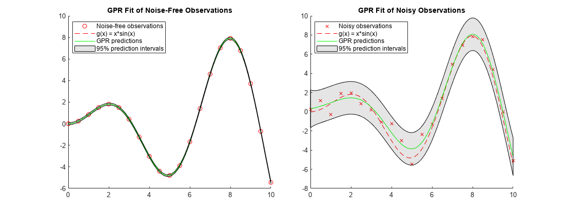
When the observations are noise free, the predicted responses of the GPR fit cross the observations. The standard deviation of the predicted response is almost zero. Therefore, the prediction intervals are very narrow. When observations include noise, the predicted responses do not cross the observations, and the prediction intervals become wide.

References

[1] Rasmussen, C. E. and C. K. I. Williams.Gaussian Processes for Machine Learning.MIT Press. Cambridge, Massachusetts, 2006.