曲面近似の評価

この例では,曲面近似を扱う方法を示します。

データの読み込みと多項式曲面による近似

loadfranke; surffit = fit([x,y],z,'poly23','normalize','on')

Linear model Poly23: surffit(x,y) = p00 + p10*x + p01*y + p20*x^2 + p11*x*y + p02*y^2 + p21*x^2*y + p12*x*y^2 + p03*y^3 where x is normalized by mean 1982 and std 868.6 and where y is normalized by mean 0.4972 and std 0.2897 Coefficients (with 95% confidence bounds): p00 = 0.4253 (0.3928, 0.4578) p10 = -0.106 (-0.1322, -0.07974) p01 = -0.4299 (-0.4775, -0.3822) p20 = 0.02104 (0.001457, 0.04062) p11 = 0.07153 (0.05409, 0.08898) p02 = -0.03084 (-0.05039, -0.01129) p21 = 0.02091 (0.001372, 0.04044) p12 = -0.0321 (-0.05164, -0.01255) p03 = 0.1216 (0.09929, 0.1439)

出力には、近似モデル方程式、近似係数、近似係数の信頼限界が表示されます。

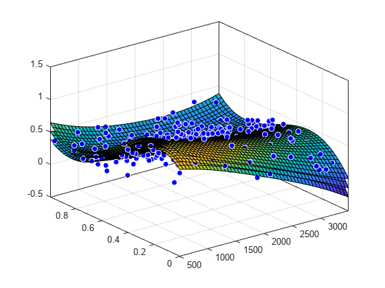
近似、データ、残差および予測限界のプロット

plot(surffit,[x,y],z)

近似の残差をプロットします。

plot(surffit,[x,y],z,'Style','Residuals')

近似の予測限界をプロットします。

plot(surffit,[x,y],z,'Style','predfunc')

指定した点での近似の評価

xとyに値を指定し、z = fittedmodel(x,y)の形式を使用すると、特定の点で近似を評価できます。

surffit(1000,0.5)

ans = 0.5673

多数の点での近似値の評価

xi = [500;1000;1200]; yi = [0.7;0.6;0.5]; surffit(xi,yi)

ans =3×10.3771 0.4064 0.5331

それらの値の予測限界を取得します。

[ci, zi] = predint(surffit,[xi,yi])

ci =3×20.0713 0.6829 0.1058 0.7069 0.2333 0.8330

zi =3×10.3771 0.4064 0.5331

モデル方程式の取得

近似名を入力し、モデル方程式、近似係数、近似係数の信頼限界を表示します。

surffit

Linear model Poly23: surffit(x,y) = p00 + p10*x + p01*y + p20*x^2 + p11*x*y + p02*y^2 + p21*x^2*y + p12*x*y^2 + p03*y^3 where x is normalized by mean 1982 and std 868.6 and where y is normalized by mean 0.4972 and std 0.2897 Coefficients (with 95% confidence bounds): p00 = 0.4253 (0.3928, 0.4578) p10 = -0.106 (-0.1322, -0.07974) p01 = -0.4299 (-0.4775, -0.3822) p20 = 0.02104 (0.001457, 0.04062) p11 = 0.07153 (0.05409, 0.08898) p02 = -0.03084 (-0.05039, -0.01129) p21 = 0.02091 (0.001372, 0.04044) p12 = -0.0321 (-0.05164, -0.01255) p03 = 0.1216 (0.09929, 0.1439)

モデル方程式のみを取得するにはformulaを使用します。

formula(surffit)

ans = 'p00 + p10*x + p01*y + p20*x^2 + p11*x*y + p02*y^2 + p21*x^2*y + p12*x*y^2 + p03*y^3'

係数の名前と値の取得

名前で係数を指定します。

p00 = surffit.p00

p00 = 0.4253

p03 = surffit.p03

p03 = 0.1216

すべての係数名を取得します。近似方程式 (f(x,y) = p00 + p10*x...など) を確認し、各係数のモデル項を調べます。

coeffnames(surffit)

ans =9x1 cell{'p00'} {'p10'} {'p01'} {'p20'} {'p11'} {'p02'} {'p21'} {'p12'} {'p03'}

すべての係数値を取得します。

coeffvalues(surffit)

ans =1×90.4253 -0.1060 -0.4299 0.0210 0.0715 -0.0308 0.0209 -0.0321 0.1216

係数の信頼限界の取得

係数の信頼限界を使用すると、近似の評価と比較に役立ちます。係数の信頼限界によって係数の精度が決まります。範囲の間隔が広いほど、不確定性が高いことを示しています。線形係数の範囲がゼロと交差する場合、これらの係数がゼロではないという確信をもてないことを意味します。あるモデル項の係数がゼロの場合、その係数は近似に寄与していません。

confint(surffit)

ans =2×90.3928 -0.1322 -0.4775 0.0015 0.0541 -0.0504 0.0014 -0.0516 0.0993 0.4578 -0.0797 -0.3822 0.0406 0.0890 -0.0113 0.0404 -0.0126 0.1439

メソッドの確認

この近似で使用できるすべてのメソッドを一覧表示します。

methods(surffit)

Methods for class sfit: argnames dependnames indepnames predint sfit category differentiate islinear probnames type coeffnames feval numargs probvalues coeffvalues fitoptions numcoeffs quad2d confint formula plot setoptions

helpコマンドを使用して fit メソッドの使用方法を確認します。

helpsfit/quad2d

QUAD2D Numerically integrate a surface fit object. Q = QUAD2D(FO, A, B, C, D) approximates the integral of the surface fit object FO over the planar region A <= x <= B and C(x) <= y <= D(x). C and D may each be a scalar, a function handle or a curve fit (CFIT) object. [Q,ERRBND] = QUAD2D(...) also returns an approximate upper bound on the absolute error, ERRBND. [Q,ERRBND] = QUAD2D(FUN,A,B,C,D,PARAM1,VAL1,PARAM2,VAL2,...) performs the integration with specified values of optional parameters. See QUAD2D for details of the upper bound and the optional parameters. See also: QUAD2D, FIT, SFIT, CFIT.

Curve Fitting Toolbox ドキュメンテーション

サポート

機械学習の課題：最適な分類モデルの選択と過適合の回避

ホワイトペーパーをダウンロード