Switching Controllers Based on Optimal Costs
This example shows how to use the "optimal cost" outport of the MPC Controller block to switch between multiple model predictive controllers whose outputs are restricted to discrete values.
Define Plant Model
The linear plant model is as follows::
plant = ss(tf({1,1},{[1 1.2 1],[1 1]}),'min');% Plant with 2 inputs and 1 output[A,B,C,D] = ssdata(plant);% Get state-space realization matrices, to be used in Simulinkx0 = [0;0;0];% Initial plant state
Design MPC Controller
Specify input and output signal types.
plant = setmpcsignals(plant,'MV',1,'MD',2);% First input is manipulated, second is measured disturbance
Design two MPC controllers with the MV constraints ofu=-1andu=1, respectively. Onlyuat the current time is quantized. The subsequent calculated control actions may be any value between -1 and 1. The controller uses a receding horizon approach so these values don't actually go to the plants.
Ts = 0.2;% Sampling timep = 20;% Prediction horizonm = 10;% Control horizonmpc1 = mpc(plant,Ts,p,m);% First MPC objectmpc2 = mpc(plant,Ts,p,m);% Second MPC object% Specify weightsmpc1.Weights = struct('MV',0,'MVRate',.3,'Output',1);% Weightsmpc2.Weights = struct('MV',0,'MVRate',.3,'Output',1);% Weights% Specify constraintsmpc1.MV = struct('Min',[-1;-1],'Max',[-1;1]);%限制操纵变量:u = 1mpc2.MV = struct('Min',[1;-1],'Max',[1;1]);% Constraints on the manipulated variable: u = 1
-->The "Weights.ManipulatedVariables" property of "mpc" object is empty. Assuming default 0.00000. -->The "Weights.ManipulatedVariablesRate" property of "mpc" object is empty. Assuming default 0.10000. -->The "Weights.OutputVariables" property of "mpc" object is empty. Assuming default 1.00000. -->The "Weights.ManipulatedVariables" property of "mpc" object is empty. Assuming default 0.00000. -->The "Weights.ManipulatedVariablesRate" property of "mpc" object is empty. Assuming default 0.10000. -->The "Weights.OutputVariables" property of "mpc" object is empty. Assuming default 1.00000.
Simulate in Simulink®
To run this example, Simulink® is required.
if~mpcchecktoolboxinstalled('simulink') disp('Simulink(R) is required to run this example.')returnend% Specify signals:Tstop = 40; ref.time = 0:Ts:(Tstop+p*Ts); ref.signals.values = double(ref.time>10)';% Step change in reference signal at time t=10md.time = ref.time; md.signals.values = double(md.time>30)';% Step change in measured disturbance signal at time t=30
Open and simulate the Simulink® model:
mdl ='mpc_optimalcost'; open_system(mdl);% Open Simulink(R) Modelsim(mdl,Tstop);% Start Simulation
——>将模型转换为离散时间。——>假设output disturbance added to measured output channel #1 is integrated white noise. -->The "Model.Noise" property of the "mpc" object is empty. Assuming white noise on each measured output channel. -->Converting model to discrete time. -->Assuming output disturbance added to measured output channel #1 is integrated white noise. -->The "Model.Noise" property of the "mpc" object is empty. Assuming white noise on each measured output channel.


Note that:
From time 0 to time 10, the control action keeps switching between MPC1 (-1) and MPC2 (+1). This is because the reference signal is 0 and it requires a controller output at 0 to reach steady state, which cannot be achieved with either MPC controller.
From time 10 to 30, MPC2 control output (+1) is chosen because the reference signal becomes +1 and it requires a controller output at +1 to reach steady state (plant gain is 1), which can be achieved by MPC2.
From time 30 to 40, control action starts switching again. This is because with the presence of measured disturbance (+1), MPC1 leads to a steady state of 0 and MPC2 leads to a steady state of +2, while the reference signal still requires +1.
Simulate Using MPCMOVE Command
Usempcmoveto perform step-by-step simulation and compute current MPC control action:
[Ad,Bd,Cd,Dd] = ssdata(c2d(plant,Ts));% Discrete-time dynamicsNsteps = round(Tstop/Ts);% Number of simulation steps
Initialize matrices for storing simulation results
YY = zeros(Nsteps+1,1); RR = zeros(Nsteps+1,1); UU = zeros(Nsteps+1,1); COST = zeros(Nsteps+1,1); x = x0;% Initial plant statext1 = mpcstate(mpc1);% Initial state of the MPC controller #1xt2 = mpcstate(mpc2);% Initial state of the MPC controller #2
Start simulation.
fortd=0:Nsteps% Construct signalsv = md.signals.values(td+1); r = ref.signals.values(td+1);% Plant equations: output updatey = Cd*x + Dd(:,2)*v;% Compute both MPC movesoptions = mpcmoveopt; options.OnlyComputeCost = true;% the last input argument tells "mpcmove" to only compute the optimal cost[u1,Info1] = mpcmove(mpc1,xt1,y,r,v,options); [u2,Info2] = mpcmove(mpc2,xt2,y,r,v,options);% Compare the resulting optimal costs and choose the input value% corresponding to the smallest costifInfo1.Cost<=Info2.Cost u = u1; cost = Info1.Cost;% Update internal MPC state to the correct valuext2.Plant = xt1.Plant; xt2.Disturbance = xt1.Disturbance; xt2.LastMove = xt1.LastMove;elseu = u2; cost = Info2.Cost;% Update internal MPC state to the correct valuext1.Plant = xt2.Plant; xt1.Disturbance = xt2.Disturbance; xt1.LastMove = xt2.LastMove;end% Store plant informationYY(td+1) = y; RR(td+1) = r; UU(td+1) = u; COST(td+1) = cost;% Plant equations: state updatex = Ad*x + Bd(:,1)*u + Bd(:,2)*v;end
Plot the results ofmpcmoveto compare with the simulation results obtained in Simulink®:
subplot(131) plot((0:Nsteps)*Ts,[YY,RR]);% Plot output and reference signalsgrid title('OV and Reference') subplot(132) plot((0:Nsteps)*Ts,UU);% Plot manipulated variablegrid title('MV') subplot(133) plot((0:Nsteps)*Ts,COST);% Plot optimal MPC value functiongrid title('Optimal cost')
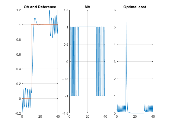
These plots resemble the plots in the scopes in the Simulink® model.
bdclose(mdl);
See Also
Related Topics
Select a Web Site
Choose a web site to get translated content where available and see local events and offers. Based on your location, we recommend that you select:.
Selectweb siteYou can also select a web site from the following list:
Americas
- América Latina(Español)
- Canada(English)
- United States(English)
Europe
- Belgium(English)
- Denmark(English)
- Deutschland(Deutsch)
- España(Español)
- Finland(English)
- France(Français)
- Ireland(English)
- Italia(Italiano)
- Luxembourg(English)
- Netherlands(English)
- Norway(English)
- Österreich(Deutsch)
- Portugal(English)
- Sweden(English)
- Switzerland
- United Kingdom(English)