Introduction

In a ground moving target indicator (GMTI) system, an airborne radar collects the returned echo from the moving target on the ground. However, the received signal contains not only the reflected echo from the target, but also the returns from the illuminated ground surface. The return from the ground is generally referred to asclutter.

The clutter return comes from all the areas illuminated by the radar beam, so it occupies all range bins and all directions. The total clutter return is often much stronger than the returned signal echo, which poses a great challenge to target detection. Clutter filtering, therefore, is a critical part of a GMTI system.

在传统MTI系统、杂物过滤而声名狼籍n takes advantage of the fact that the ground does not move. Thus, the clutter occupies the zero Doppler bin in the Doppler spectrum. This principle leads to many Doppler-based clutter filtering techniques, such as pulse canceller. Interested readers can refer toGround Clutter Mitigation with Moving Target Indication (MTI) Radar(Radar Toolbox)for a detailed example of the pulse canceller. When the radar platform itself is also moving, such as in a plane, the Doppler component from the ground return is no longer zero. In addition, the Doppler components of clutter returns are angle dependent. In this case, the clutter return is likely to have energy across the Doppler spectrum. Therefore, the clutter cannot be filtered only with respect to Doppler frequency.

Jamming is another significant interference source that is often present in the received signal. The simplest form of jamming is a barrage jammer, which is strong, continuous white noise directed toward the radar receiver so that the receiver cannot easily detect the target return. The jammer is usually at a specific location, and the jamming signal is therefore associated with a specific direction. However, because of the white noise nature of the jammer, the received jamming signal occupies the entire Doppler band.

STAP techniques filter the signal in both the angular and Doppler domains (thus, the name "space-time adaptive processing") to suppress the clutter and jammer returns. In the following sections, we simulate returns from target, clutter, and jammer and illustrate how STAP techniques filter the interference from the received signal.

System Setup

We first define a radar system, starting from the system built in the exampleSimulating Test Signals for a Radar Receiver.

loadBasicMonostaticRadarExampleData.mat;% Load monostatic pulse radar

Antenna Definition

Assume that the antenna element has an isotropic response in the front hemisphere and all zeros in the back hemisphere. The operating frequency range is set to 8 to 12 GHz to match the 10 GHz operating frequency of the system.

antenna = phased.IsotropicAntennaElement...('FrequencyRange',[8e9 12e9],'BackBaffled',true);% Baffled Isotropic

Define a 6-element ULA with a custom element pattern. The element spacing is assumed to be one half the wavelength of the waveform.

fc = radiator.OperatingFrequency; c = radiator.PropagationSpeed; lambda = c/fc; ula = phased.ULA('Element',antenna,'NumElements',6,...'ElementSpacing', lambda/2); pattern(ula,fc,'PropagationSpeed',c,'Type','powerdb') title('6-element Baffled ULA Response Pattern') view(60,50)

Radar Setup

Next, mount the antenna array on the radiator/collector. Then, define the radar motion. The radar system is mounted on a plane that flies 1000 meters above the ground. The plane is flying along the array axis of the ULA at a speed such that it travels a half element spacing of the array during one pulse interval. (An explanation of such a setting is provided in the DPCA technique section that follows.)

radiator.Sensor = ula; collector.Sensor = ula; sensormotion = phased.Platform('InitialPosition',[0; 0; 1000]); arrayAxis = [0; 1; 0]; prf = waveform.PRF; vr = ula.ElementSpacing*prf;% in [m/s]sensormotion.Velocity = vr/2*arrayAxis;

Target

Next, define a nonfluctuating target with a radar cross section of 1 square meter moving on the ground.

target = phased.RadarTarget('Model','Nonfluctuating','MeanRCS',1,...'OperatingFrequency', fc); tgtmotion = phased.Platform('InitialPosition',[1000; 1000; 0],...'Velocity',[30; 30; 0]);

Jammer

The target returns the desired signal; however, several interferences are also present in the received signal. If Radar Toolbox is available, please set the varaiblehasRadarToolboxto true to define a simple barrage jammer with an effective radiated power of 100 watts. Otherwise, the simulation will use a saved jammer signal.

hasRadarToolbox = false; Fs = waveform.SampleRate; rngbin = c/2*(0:1/Fs:1/prf-1/Fs).';ifhasRadarToolbox jammer = barrageJammer('ERP',100); jammer.SamplesPerFrame = numel(rngbin); jammermotion = phased.Platform('InitialPosition',[1000; 1732; 1000]);end

Clutter

在这个示例中,我们使用的模拟杂波constant gamma model with a gamma value of -15 dB. Literature shows that such a gamma value can be used to model terrain covered by woods. For each range, the clutter return can be thought of as a combination of the returns from many small clutter patches on that range ring. Since the antenna is back baffled, the clutter contribution is only from the front. To simplify the computation, use an azimuth width of 10 degrees for each patch. Again, if Radar Toolbox is not available, the simulation will use a saved clutter signal.

ifhasRadarToolbox Rmax = 5000; Azcov = 120; clutter = constantGammaClutter('Sensor',ula,'SampleRate',Fs,...'Gamma',-15,'PlatformHeight',1000,...'OperatingFrequency',fc,...'PropagationSpeed',c,...'PRF',prf,...'TransmitERP',transmitter.PeakPower*db2pow(transmitter.Gain),...'PlatformSpeed',norm(sensormotion.Velocity),...'PlatformDirection',[90;0],...'ClutterMaxRange', Rmax,...'ClutterAzimuthSpan',Azcov,...'PatchAzimuthSpan',10,...'OutputFormat','Pulses');end

Propagation Paths

Finally, create a free space environment to represent the target and jammer paths. Because we are using a monostatic radar system, the target channel is set to simulate two-way propagation delays. The jammer path computes only one-way propagation delays.

tgtchannel = phased.FreeSpace('TwoWayPropagation',true,'SampleRate',Fs,...'OperatingFrequency', fc); jammerchannel = phased.FreeSpace('TwoWayPropagation',false,...'SampleRate',Fs,'OperatingFrequency', fc);

Simulation Loop

We are now ready to simulate the returns. Collect 10 pulses before processing. The seed of the random number generator from the jammer model is set to a constant to get reproducible results.

numpulse = 10;% Number of pulsestsig = zeros(size(rngbin,1), ula.NumElements, numpulse); jsig = tsig; tjcsig = tsig; tcsig = tsig; csig = tsig;ifhasRadarToolbox jammer.SeedSource ='Property'; jammer.Seed = 5; clutter.SeedSource ='Property'; clutter.Seed = 5;elseloadSTAPIntroExampleData;endform = 1:numpulse% Update sensor, target and calculate target angle as seen by the sensor[sensorpos,sensorvel] = sensormotion(1/prf); [tgtpos,tgtvel] = tgtmotion(1/prf); [~,tgtang] = rangeangle(tgtpos,sensorpos);% Update jammer and calculate the jammer angles as seen by the sensorifhasRadarToolbox [jampos,jamvel] = jammermotion(1/prf); [~,jamang] = rangeangle(jampos,sensorpos);end% Simulate propagation of pulse in direction of targetspulse = waveform(); [pulse,txstatus] = transmitter(pulse); pulse = radiator(pulse,tgtang); pulse = tgtchannel(pulse,sensorpos,tgtpos,sensorvel,tgtvel);% Collect target returns at sensorpulse = target(pulse); tsig(:,:,m) = collector(pulse,tgtang);% Collect jammer and clutter signal at sensorifhasRadarToolbox jamsig = jammer(); jamsig = jammerchannel(jamsig,jampos,sensorpos,jamvel,sensorvel); jsig(:,:,m) = collector(jamsig,jamang); csig(:,:,m) = clutter();end% Receive collected signalstjcsig(:,:,m) = receiver(tsig(:,:,m)+jsig(:,:,m)+csig(:,:,m),...~(txstatus>0));% Target + jammer + cluttertcsig(:,:,m) = receiver(tsig(:,:,m)+csig(:,:,m),...~(txstatus>0));% Target + cluttertsig(:,:,m) = receiver(tsig(:,:,m),...~(txstatus>0));% Target echo onlyend

True Target Range, Angle and Doppler

The target azimuth angle is 45 degrees, and the elevation angle is about -35.27 degrees.

tgtLocation = global2localcoord(tgtpos,'rs',sensorpos); tgtAzAngle = tgtLocation(1)

tgtAzAngle = 44.9981

tgtElAngle = tgtLocation(2)

tgtElAngle = -35.2651

The target range is 1732 m.

tgtRng = tgtLocation(3)

tgtRng = 1.7320e+03

The target Doppler normalized frequency is about 0.21.

sp = radialspeed(tgtpos, tgtmotion.Velocity,...sensorpos, sensormotion.Velocity); tgtDp = 2*speed2dop(sp,lambda);% Round trip DopplertgtDp/prf

ans = 0.2116

The total received signal contains returns from the target, clutter and jammer combined. The signal is a data cube with three dimensions (range bins x number of elements x number of pulses). Notice that the clutter return dominates the total return and masks the target return. We cannot detect the target (blue vertical line) without further processing at this stage.

ReceivePulse = tjcsig; plot([tgtRng tgtRng],[0 0.01],rngbin,abs(ReceivePulse(:,:,1))); xlabel('Range (m)'), ylabel('Magnitude'); title('Signals collected by the ULA within the first pulse interval')

Now, examine the returns in 2-D angle Doppler (or space-time) domain. In general, the response is generated by scanning all ranges and azimuth angles for a given elevation angle. Because we know exactly where the target is, we can calculate its range and elevation angle with respect to the antenna array.

tgtCellIdx = val2ind(tgtRng,c/(2*Fs)); snapshot = shiftdim(ReceivePulse(tgtCellIdx,:,:));% Remove singleton dimangdopresp = phased.AngleDopplerResponse('SensorArray',ula,...'OperatingFrequency',fc,'PropagationSpeed',c,...'PRF',prf,'ElevationAngle',tgtElAngle); plotResponse(angdopresp,snapshot,'NormalizeDoppler',true); text(tgtAzAngle,tgtDp/prf,'+ Target')

If we look at the angle Doppler response which is dominated by the clutter return, we see that the clutter return occupies not only the zero Doppler, but also other Doppler bins. The Doppler of the clutter return is also a function of the angle. The clutter return looks like a diagonal line in the entire angle Doppler space. Such a line is often referred to asclutter ridge. The received jammer signal is white noise, which spreads over the entire Doppler spectrum at a particular angle, around 60 degrees.

Clutter Suppression with a DPCA Canceller

The displaced phase center antenna (DPCA) algorithm is often considered to be the first STAP algorithm. This algorithm uses the shifted aperture to compensate for the platform motion so that the clutter return does not change from pulse to pulse. Thus, this algorithm can remove the clutter via a simple subtraction of two consecutive pulses.

A DPCA canceller is often used on ULAs but requires special platform motion conditions. The platform must move along the antenna's array axis and at a speed such that during one pulse interval, the platform travels exactly half of the element spacing. The system used here is set up, as described in earlier sections, to meet these conditions.

Assume that N is the number of ULA elements. The clutter return received at antenna 1 through antenna N-1 during the first pulse is the same as the clutter return received at antenna 2 through antenna N during the second pulse. By subtracting the pulses received at these two subarrays during the two pulse intervals, the clutter can be cancelled out. The cost of this method is an aperture that is one element smaller than the original array.

Now, define a DPCA canceller. The algorithm may need to search through all combinations of angle and Doppler to locate a target, but for the example, because we know exactly where the target is, we can direct our processor to that point.

rxmainlobedir = [0; 0]; stapdpca = phased.DPCACanceller('SensorArray',ula,'PRF',prf,...'PropagationSpeed',c,'OperatingFrequency',fc,...'Direction',rxmainlobedir,'Doppler',tgtDp,...'WeightsOutputPort',true)

stapdpca = phased.DPCACanceller with properties: SensorArray: [1x1 phased.ULA] PropagationSpeed: 299792458 OperatingFrequency: 1.0000e+10 PRFSource: 'Property' PRF: 2.9979e+04 DirectionSource: 'Property' Direction: [2x1 double] NumPhaseShifterBits: 0 DopplerSource: 'Property' Doppler: 6.3429e+03 WeightsOutputPort: true PreDopplerOutput: false

First, apply the DPCA canceller to both the target return and the clutter return.

ReceivePulse = tcsig; [y,w] = stapdpca(ReceivePulse,tgtCellIdx);

The processed data combines all information in space and across the pulses to become a single pulse. Next, examine the processed signal in the time domain.

plot([tgtRng tgtRng],[0 1.2e-5],rngbin,abs(y)); xlabel('Range (m)'), ylabel('Magnitude'); title('DPCA Canceller Output (no Jammer)')

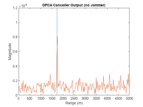
The signal now is clearly distinguishable from the noise and the clutter has been filtered out. From the angle Doppler response of the DPCA processor weights below, we can also see that the weights produce a deep null along the clutter ridge.

angdopresp.ElevationAngle = 0; plotResponse(angdopresp,w,'NormalizeDoppler',true); title('DPCA Weights Angle Doppler Response at 0 degrees Elevation')

Although the results obtained by DPCA are very good, the radar platform has to satisfy very strict requirements in its movement to use this technique. Also, the DPCA technique cannot suppress the jammer interference.

Applying DPCA processing to the total signal produces the result shown in the following figure. We can see that DPCA cannot filter the jammer from the signal. The resulting angle Doppler pattern of the weights is the same as before. Thus, the processor cannot adapt to the newly added jammer interference.

ReceivePulse = tjcsig; [y,w] = stapdpca(ReceivePulse,tgtCellIdx); plot([tgtRng tgtRng],[0 8e-4],rngbin,abs(y)); xlabel('Range (m)'), ylabel('Magnitude'); title('DPCA Canceller Output (with Jammer)')

plotResponse(angdopresp,w,'NormalizeDoppler',true); title('DPCA Weights Angle Doppler Response at 0 degrees Elevation')

Clutter and Jammer Suppression with an SMI Beamformer

To suppress the clutter and jammer simultaneously, we need a more sophisticated algorithm. The optimum receiver weights, when the interference is Gaussian-distributed, are given by [1]

wherekis a scalar factor,Ris the space-time covariance matrix of the interference signal, ands是所需的时空控制向量。穰的ct information ofRis often unavailable, so we will use the sample matrix inversion (SMI) algorithm. The algorithm estimatesRfrom training-cell samples and then uses it in the aforementioned equation.

现在,定义一个重度beamformer并应用它signal. In addition to the information needed in DPCA, the SMI beamformer needs to know the number of guard cells and the number of training cells. The algorithm uses the samples in the training cells to estimate the interference. Thus, we should not use the cells that are close to the target cell for the estimates because they may contain some target information, i.e., we should define guard cells. The number of guard cells must be an even number to be split equally in front of and behind the target cell. The number of training cells also must be an even number and split equally in front of and behind the target. Normally, the larger the number of training cells, the better the interference estimate.

tgtAngle = [tgtAzAngle; tgtElAngle]; stapsmi = phased.STAPSMIBeamformer('SensorArray', ula,'PRF', prf,...'PropagationSpeed', c,'OperatingFrequency', fc,...'Direction', tgtAngle,'Doppler', tgtDp,...'WeightsOutputPort', true,...'NumGuardCells', 4,'NumTrainingCells', 100)

stapsmi = phased.STAPSMIBeamformer with properties: SensorArray: [1x1 phased.ULA] PropagationSpeed: 299792458 OperatingFrequency: 1.0000e+10 PRFSource: 'Property' PRF: 2.9979e+04 DirectionSource: 'Property' Direction: [2x1 double] NumPhaseShifterBits: 0 DopplerSource: 'Property' Doppler: 6.3429e+03 NumGuardCells: 4 NumTrainingCells: 100 WeightsOutputPort: true

[y,w] = stapsmi(ReceivePulse,tgtCellIdx); plot([tgtRng tgtRng],[0 2e-6],rngbin,abs(y)); xlabel('Range (m)'), ylabel('Magnitude'); title('SMI Beamformer Output (with Jammer)')

plotResponse(angdopresp,w,'NormalizeDoppler',true); title('SMI Weights Angle Doppler Response at 0 degrees Elevation')

The result shows that an SMI beamformer can distinguish signals from both the clutter and the jammer. The angle Doppler pattern of the SMI weights shows a deep null along the jammer direction.

SMI provides the maximum degrees of freedom, and hence, the maximum gain among all STAP algorithms. It is often used as a baseline for comparing different STAP algorithms.

Reducing the Computation Cost with an ADPCA Canceller

Although SMI is the optimum STAP algorithm, it has several innate drawbacks, including a high computation cost because it uses the full dimension data of each cell. More importantly, SMI requires a stationary environment across many pulses. This kind of environment is not often found in real applications. Therefore, many reduced dimension STAP algorithms have been proposed.

An adaptive DPCA (ADPCA) canceller filters out the clutter in the same manner as DPCA, but it also has the capability to suppress the jammer as it estimates the interference covariance matrix using two consecutive pulses. Because there are only two pulses involved, the computation is greatly reduced. In addition, because the algorithm is adapted to the interference, it can also tolerate some motion disturbance.

Now, define an ADPCA canceller, and then apply it to the received signal.

stapadpca =分阶段。ADPCACanceller ('SensorArray', ula,'PRF', prf,...'PropagationSpeed', c,'OperatingFrequency', fc,...'Direction', rxmainlobedir,'Doppler', tgtDp,...'WeightsOutputPort', true,...'NumGuardCells', 4,'NumTrainingCells', 100)

stapadpca =分阶段。ADPCACanceller with properties: SensorArray: [1x1 phased.ULA] PropagationSpeed: 299792458 OperatingFrequency: 1.0000e+10 PRFSource: 'Property' PRF: 2.9979e+04 DirectionSource: 'Property' Direction: [2x1 double] NumPhaseShifterBits: 0 DopplerSource: 'Property' Doppler: 6.3429e+03 NumGuardCells: 4 NumTrainingCells: 100 WeightsOutputPort: true PreDopplerOutput: false

[y,w] = stapadpca(ReceivePulse,tgtCellIdx); plot([tgtRng tgtRng],[0 2e-6],rngbin,abs(y)); xlabel('Range (m)'), ylabel('Magnitude'); title('ADPCA Canceller Output (with Jammer)')

plotResponse(angdopresp,w,'NormalizeDoppler',true); title('ADPCA Weights Angle Doppler Response at 0 degrees Elevation')

The time domain plot shows that the signal is successfully recovered. The angle Doppler response of the ADPCA weights is similar to the one produced by the SMI weights.

Summary

This example presented a brief introduction to space-time adaptive processing and illustrated how to use different STAP algorithms, namely, SMI, DPCA, and ADPCA, to suppress clutter and jammer interference in the received pulses.

Reference

[1] J. R. Guerci,Space-Time Adaptive Processing for Radar, Artech House, 2003