polyplotdocumentation
This function plots a polynomial fit to scatteredx,ydata. This function can be used to easily add a linear trend line or other polynomial fit to a data plot.
Back to Climate Data Tools Contents.
Contents
Syntax
polyplot(x,y) polyplot(x,y,n) polyplot(...,'weight',w) polyplot(...,'Name',Value,...) polyplot(...,'error') [h,p,delta] = polyplot(...)
Description
polyplot(x,y)places a least-squares linear trend line through scatteredx,ydata.
polyplot(x,y,n)specifies the degreenof the polynomial fit to thex,ydata. Defaultnis1.
polyplot(...,'weight',w)uses thepolyfitw函数允许加权最小二乘相吻合。
polyplot(...,'Name',Value,...)formats linestyle usingLineSpecproperty name-value pairs (e.g.,'linewidth',3). If 'error' bounds are plotted, onlyboundedlineproperties are accepted.
polyplot(...,'error')includes lines corresponding to approximately +/- 1 standard deviation of errorsdelta. At least 50% of data should lie within the bounds of error lines. Error bounds are plotted withboundedline.
h = polyplot(...)returns handle(s)hof plotted objects.
Examples
Given some data:
x = 1:100; y = 12 - 0.01*x.^2 + 3*x + sind(x) + 30*rand(size(x));
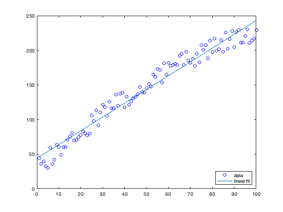
Plot the data and add a simple linear trend line:
plot(x,y,'bo') holdonpolyplot(x,y); legend('data','linear fit','location','southeast')
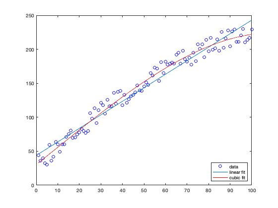
Instead of a linear trend, make it a cubic fit:
polyplot(x,y,3,'r'); legend('data','linear fit','cubic fit','location','southeast')
Add a fat, black 7th-order polynomial fit:
polyplot(x,y,7,'k','linewidth',4); legend('data','linear fit','cubic fit',...'7^{th} order fit','location','southeast')

Same as above, but with +/- 1 standard deviation of error lines:
figure h(1) = plot(x,y,'bo'); holdonh(2:3) = polyplot(x,y,7,'r','error','alpha'); legend(h,'data','7^{th} order fit','\pm1\sigma','location','southeast')

Author Info
Thepolyplotfunction and supporting documentation were created byChad A. Greeneof the University of Texas at Austin'sInstitute for Geophysics (UTIG). January 2015. Adapted for CDT in 2019.