Designing PID for Disturbance Rejection with PID Tuner
This example shows how to design a PI controller with good disturbance rejection performance using the PID Tuner tool. The example also shows how to design an ISA-PID controller for both good disturbance rejection and good reference tracking.
Launching the PID Tuner with Initial PID Design
The plant model is
G = zpk(-5,[-1 -2 -3 -4],6,'OutputDelay',1); G.InputName ='u'; G.OutputName ='y';
Use the following command to launch the PID Tuner to design a PI controller in parallel form for plant G.
pidtool(G,'pi')
The PID Tuner automatically designs an initial PI controller. Click "Show parameters" button to display the controller gains and performance metrics.


For step reference tracking, the settling time is about 12 seconds and the overshoot is about 6.3 percent, which is acceptable for this example.
Tuning PID for Disturbance Rejection
Assume that a step disturbance occurs at the plant input and the main purpose of the PI controller is to reject this disturbance quickly. In the rest of this section, we will show how to design the PI controller for better disturbance rejection in the PID Tuner. We also expect that the reference tracking performance is degraded as disturbance rejection performance improves.
Because the attenuation of low frequency disturbance is inversely proportional to integral gain Ki, maximizing the integral gain is a useful heuristic to obtain a PI controller with good disturbance rejection. For background, see Karl Astrom et al., "Advanced PID Control", Chapter 4 "Controller Design", 2006, The ISA Society.
ClickAdd Plot andselectInput disturbance rejectionto plot the input disturbance step response. The peak deviation is about 1 and it settles to less than 0.1 in about 9 seconds.


Tile the plots to show both the reference tracking and input disturbance responses. Move the response time slider to the right to increase the response speed (open loop bandwidth). The Ki gain in theController parameterstable first increases and then decreases, with the maximum value occurring at 0.3. When Ki is 0.3, the peak deviation is reduced to 0.9 (about 10% improvement) and it settles to less than 0.1 in about 6.7 seconds (about 25% improvement).


Because we increased the bandwidth, the step reference tracking response becomes more oscillatory. Additionally the overshoot exceeds 15 percent, which is usually unacceptable. This type of performance trade off between reference tracking and disturbance rejection often exists because a single PID controller is not able to satisfy both design goals at the same time.
ClickExportto export the designed PI controller to the MATLAB Workspace. The controller is represented by a PID object and you need it to create an ISA-PID controller in the next section.

You can also manually create the same PI controller in MATLAB Workspace by using thepidcommand. In this command you can directly specify the Kp and Ki gains obtained from the parameter table of the PID Tuner.
C = pid(0.64362,0.30314); C.InputName ='e'; C.OutputName ='u'; C
C = 1 Kp + Ki * --- s with Kp = 0.644, Ki = 0.303 Continuous-time PI controller in parallel form.
Extending PID controller to ISA-PID Controller
A simple solution to make a PI controller perform well for both reference tracking and disturbance rejection is to upgrade it to an ISA-PID controller. It improves reference tracking response by providing an additional tuning parametersbthat allows independent control of the impact of the reference signal on the proportional action.

In the above ISA-PID structure, there is a feedback controller C and a feed-forward filter F. In this example, C is a regular PI controller in parallel form that can be represented by a PID object:
F is a pre-filter that involves Kp and Ki gains from C plus the setpoint weightb:
Therefore the ISA-PID controller has two inputs (r and y) and one output (u).
Set-point weightbis a real number between 0 and 1. When it decreases, the overshoot in the reference tracking response is reduced. In this example,bis chosen to be 0.7.
b = 0.7;% The following code constructs an ISA-PID from F and CF = tf([b*C.Kp C.Ki],[C.Kp C.Ki]); F.InputName ='r'; F.OutputName ='uf'; Sum = sumblk('e','uf','y','+-'); ISAPID = connect(C,F,Sum,{'r','y'},'u'); tf(ISAPID)
ans = From input "r" to output "u": 0.4505 s^2 + 0.5153 s + 0.1428 ------------------------------ s^2 + 0.471 s From input "y" to output "u": -0.6436 s - 0.3031 ------------------ s Continuous-time transfer function.
Compare Performance
The reference tracking response with ISA-PID controller has much less overshoot because setpoint weightbreduces overshoot.
% Closed-loop system with PI controller for reference trackingsys1 = feedback(G*C,1);% Closed-loop system with ISA-PID controllersys2 = connect(ISAPID,G,{'r','u'},'y');% Compare responsesstep(sys1,'r-',sys2(1),“b”。); legend('show','location','southeast') title('Reference Tracking')

The disturbance rejection responses are the same because setpoint weightbonly affects reference tracking.
% Closed-loop system with PI controller for disturbance rejectionsys1 = feedback(G,C);% Compare responsesstep(sys1,'r-',sys2(2),“b”。); legend('PID','ISA-PID'); title('Disturbance Rejection')

Select a Web Site
Choose a web site to get translated content where available and see local events and offers. Based on your location, we recommend that you select:.
Selectweb siteYou can also select a web site from the following list:
Americas
- América Latina(Español)
- Canada(English)
- United States(English)
Europe
- Belgium(English)
- Denmark(English)
- Deutschland(Deutsch)
- España(Español)
- Finland(English)
- France(Français)
- Ireland(English)
- Italia(Italiano)
- Luxembourg(English)
- Netherlands(English)
- Norway(English)
- Österreich(Deutsch)
- Portugal(English)
- Sweden(English)
- Switzerland
- United Kingdom(English)