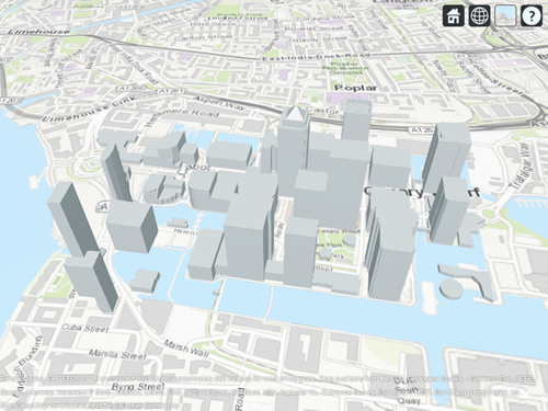
Import and Visualize Buildings Data

导入一个OpenStreetMap (. om) file corresponding to Canary Wharf in London, UK. The file was downloaded fromhttps://www.openstreetmap.org, which provides access to crowd-sourced map data all over the world. The data is licensed under the Open Data Commons Open Database License (ODbL),https://opendatacommons.org/licenses/odbl/. The buildings information contained within the OpenStreetMap file is imported and visualized in Site Viewer.

观众= siteviewer("Buildings","canarywharf.osm","Basemap","topographic");

Define Transmitter Site

Define a transmitter site to model a small cell scenario in a dense urban environment. The transmitter site represents a base station that is placed on a pole servicing the surrounding area which includes a neighboring park. The transmitter uses the default isotropic antenna, and operates at a carrier frequency of 28 GHz with a power level of 5 W.

tx = txsite("Name","Small cell transmitter",..."Latitude",51.50375,..."Longitude",-0.01843,..."AntennaHeight",10,..."TransmitterPower",5,..."TransmitterFrequency",28e9); show(tx)

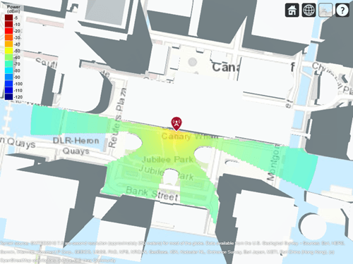
View Coverage Map for Line-of-Sight Propagation

Create a ray tracing propagation model using the shooting and bouncing ray (SBR) method. The SBR propagation model uses ray tracing analysis to compute propagation paths and their corresponding path losses. Path loss is calculated from free-space loss and reflection loss due to material, and antenna polarization loss.

Set the maximum number of reflections to 0 in order to limit the initial analysis to line-of-sight propagation paths only. Set the building and terrain material types to model perfect reflection.

rtpm = propagationModel("raytracing",..."Method","sbr",..."MaxNumReflections",0,..."BuildingsMaterial","perfect-reflector",..."TerrainMaterial","perfect-reflector");

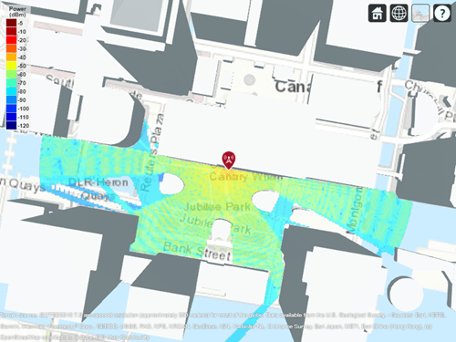
View the corresponding coverage map for a maximum range of 250 meters from the base station. The coverage map shows received power for a receiver at each ground location but is not computed for building tops or sides.

coverage(tx,rtpm,..."SignalStrengths",-120:-5,..."MaxRange",250,..."Resolution",3,..."Transparency",0.6)

Define Receiver Site in Non-Line-of-Sight Location

The coverage map for line-of-sight propagation shows shadowing due to obstructions. Define a receiver site to model a mobile receiver in an obstructed location. Plot the line-of-sight path to show the obstructed path from the transmitter to the receiver.

rx = rxsite("Name","Small cell receiver",..."Latitude",51.50216,..."Longitude",-0.01769,..."AntennaHeight",1); los(tx,rx)

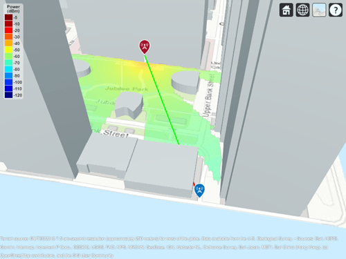
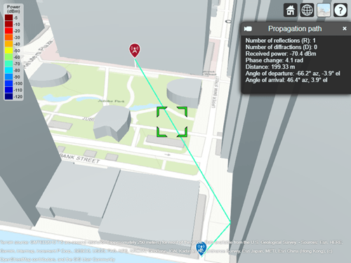
Plot Propagation Path using Ray Tracing

Adjust the ray tracing propagation model to include single-reflection paths, and plot the rays. The result shows signal propagation along a single-reflection path. The path does not end exactly at the receiver site because the SBR ray tracing method computes approximate paths. Select the plotted path to view the corresponding propagation characteristics, which include received power, phase change, distance, and angles of departure and arrival.

rtpm.MaxNumReflections = 1; clearMap(viewer) raytrace(tx,rx,rtpm)

Analyze Signal Strength and Effect of Materials

Compute the received power using the propagation model which was previously configured to model perfect reflection. Then assign a more realistic material type and re-compute the received power. Update the rays shown in Site Viewer. The use of realistic material reflection results in about 8 dB of power loss compared to perfect reflection.

ss = sigstrength(rx,tx,rtpm); disp("Received power using perfect reflection: "+ ss +" dBm")

Received power using perfect reflection: -70.3924 dBm

rtpm.BuildingsMaterial ="concrete"; rtpm.TerrainMaterial ="concrete"; raytrace(tx,rx,rtpm) ss = sigstrength(rx,tx,rtpm); disp("Received power using concrete materials: "+ ss +" dBm")

Received power using concrete materials: -78.9591 dBm

Include Weather Loss

Adding weather impairments to the propagation model and re-computing the received power results in another 1.5 dB of loss.

rtPlusWeather =...rtpm + propagationModel("gas") + propagationModel("rain"); raytrace(tx,rx,rtPlusWeather) ss = sigstrength(rx,tx,rtPlusWeather); disp("Received power including weather loss: "+ ss +" dBm")

Received power including weather loss: -80.4766 dBm

Plot Propagation Paths including Two Reflections

Expand the point-to-point analysis to include two-reflection paths and choose a smaller angular separation between launched rays for the SBR method. The visualization shows two clusters of propagation paths and the total received power increases by approximately 3 dB compared to the single-reflection paths.

rtPlusWeather.PropagationModels(1).MaxNumReflections = 2; rtPlusWeather.PropagationModels(1).AngularSeparation ="low"; ss = sigstrength(rx, tx, rtPlusWeather); disp("Received power with two-reflection paths: "+ ss +" dBm")

Received power with two-reflection paths: -77.1445 dBm

clearMap(viewer) raytrace(tx,rx,rtPlusWeather);

视图与单个反射路径覆盖率地图

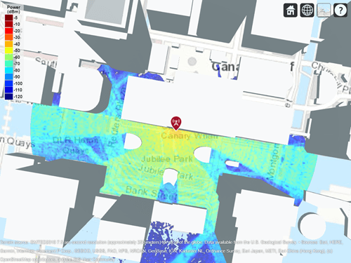
Use the configured propagation model and re-generate a coverage map including single-reflection paths and weather impairments. Code to re-generate the coverage results is included but commented out. The results, producible by running the code, are loaded from file to save several minutes of computation time in the example presentation. The resultant coverage map shows received power in the area around the non-line-of-site receiver analyzed above.

rtPlusWeather.PropagationModels(1).MaxNumReflections = 1; clearMap(viewer)

Load coverage results and plot. Coverage results were generated using commented coverage call below, which takes a few minutes to complete.

show(tx) coverageResults = load("coverageResults.mat"); contour(coverageResults.propDataSingleRef,..."Type","power",..."Transparency",0.6)% coverage(tx,rtPlusWeather, ...% "SignalStrengths",-120:-5, ...% "MaxRange", 250, ...% "Resolution",2, ...% "Transparency",0.6);

View Coverage Map with Four-Reflection

Account for more propagation paths and generate a more accurate coverage map by increasing the maximum number of reflections for the ray tracing analysis to 4. Visualize a pre-computed coverage map again which shows nearly full coverage for the area around the transmitter site.

rtPlusWeather.PropagationModels(1).MaxNumReflections = 4; clearMap(viewer)

Use pre-loaded coverage results to plot. Coverage results were generated using commented coverage call below, which may take a few hours to complete depending on the computer hardware.

show(tx) contour(coverageResults.propDataFourRef,..."Type","power",..."Transparency",0.6)% coverage(tx,rtPlusWeather, ...% "SignalStrengths",-120:-5, ...% "MaxRange", 250, ...% "Resolution",2, ...% "Transparency",0.6);

Use Beam Steering to Enhance Received Power

Many modern communications systems use techniques to steer the transmitter antenna to achieve optimal link quality. This section uses Phased Array System Toolbox™ to optimally steer a beam to maximize received power for a non-line-of-sight link.

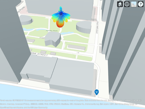
Define a custom antenna from Report ITU-R M.2412[1]for evaluating 5G radio technologies. Create an 8-by-8 uniform rectangular array from the element pattern defined in Section 8.5 of the report, point it south, and view the radiation pattern.

tx.Antenna = helperM2412PhasedArray(tx.TransmitterFrequency); tx.AntennaAngle = -90; clearMap(viewer) show(rx) pattern(tx,"Transparency",0.6) hide(tx)

Callraytracewith an output to access the rays that were computed. The returnedcomm.Rayobjects include both the geometric and propagation-related characteristics of each ray.

rtPlusWeather.PropagationModels(1).MaxNumReflections = 1; ray = raytrace(tx,rx,rtPlusWeather); disp(ray{1})

Ray with properties: PathSpecification: 'Locations' CoordinateSystem: 'Geographic' TransmitterLocation: [3×1 double] ReceiverLocation: [3×1 double] LineOfSight: 0 Interactions: [1×1 struct] Frequency: 2.8000e+10 PathLossSource: 'Custom' PathLoss: 117.4546 PhaseShift: 3.8170 Read-only properties: PropagationDelay: 6.6489e-07 PropagationDistance: 199.3293 AngleOfDeparture: [2×1 double] AngleOfArrival: [2×1 double] NumInteractions: 1

Get the angle-of-departure for the single-reflection path and apply this angle to steer the antenna in the optimal direction to achieve higher received power. The angle-of-departure azimuth is offset by the physical antenna angle azimuth to convert it to the steering vector azimuth defined in the local coordinate system of the phased array antenna.

aod = ray{1}.AngleOfDeparture; steeringaz = wrapTo180(aod(1)-tx.AntennaAngle(1)); steeringVector = phased.SteeringVector("SensorArray",tx.Antenna); sv = steeringVector(tx.TransmitterFrequency,[steeringaz;aod(2)]); tx.Antenna.Taper = conj(sv);

Plot the radiation pattern to show the antenna energy directed along the propagation path. The new received power increases by about 20 dB. The increased received power corresponds to the peak gain of the antenna.

pattern(tx,"Transparency",0.6) raytrace(tx,rx,rtPlusWeather); hide(tx) ss = sigstrength(rx, tx, rtPlusWeather); disp("Received power with beam steering: "+ ss +" dBm")

Received power with beam steering: -57.5126 dBm

Conclusion

This example used ray tracing for link and coverage analysis in an urban environment. The analysis shows:

This example analyzed received power and path loss for links and coverage. To see how to use ray tracing to configure a channel model for link-level simulation, see theIndoor MIMO-OFDM Communication Link using Ray Tracingexample.

References

[1] Report ITU-R M.2412, "Guidelines for evaluation of radio interface technologies for IMT-2020", 2017.https://www.itu.int/pub/R-REP-M.2412