摆钟组件

此示例的植物是以下的摆/卡车组件，其中zis the cart position andThetais the pendulum angle.

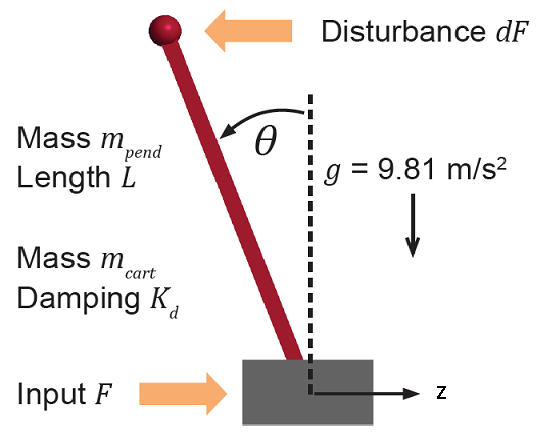
该系统的操纵变量是可变力F在购物车上行动。力的范围在-100至100之间（假定MKS单位）。控制器需要在将购物车移至新位置或通过冲动干扰将钟摆推动到前方时保持钟摆直立DFapplied at the upper end of the inverted pendulum.

控制目标

假设摆锤/购物车的以下初始条件：

控制目标是：

这upright position is an unstable equilibrium for the inverted pendulum, which makes the control task more challenging.

随时间变化的MPC的选择

In控制手推车上的倒摆，单个MPC控制器能够将购物车移至新位置-10and10。However, if you increase the step setpoint change to20，摆在过渡过程中未能恢复其直立位置。

To reach the longer distance within the same rise time, the controller applies more force to the cart at the beginning. As a result, the pendulum is displaced from its upright position by a larger angle, such as60degrees. At such angles, the plant dynamics differ significantly from the LTI predictive model obtained atTheta=0。一种s a result, errors in the prediction of plant behavior exceed what the built-in MPC robustness can handle, and the controller fails to perform properly.

To avoid the pendulum falling, a simple workaround is to restrict pendulum displacement by adding soft output constraints toThetaand reducing the ECR weight (from the default value of 1e5 to 100) to soften the constraints.

mpcobj.OV(2).Min = -pi/2; mpcobj.OV(2).Max = pi/2; mpcobj.Weights.ECR = 100;

但是，使用这些新的控制器设置，不再有可能在所需的上升时间内达到更长的距离。换句话说，牺牲控制器的性能是为了避免违反软输出约束。

To move the cart to a new position between-20and20在保持相同的上升时间的同时，控制器需要以不同的角度具有更准确的模型，以便控制器可以使用它们来更好地预测。自适应MPC使您可以通过在运行时更新线性时变植物模型来解决非线性控制问题。

Control Structure

For this example, use a single LTV MPC controller with:

mdlMPC ='mpc_pendcartLTVMPC';Open_System（MDLMPC）;

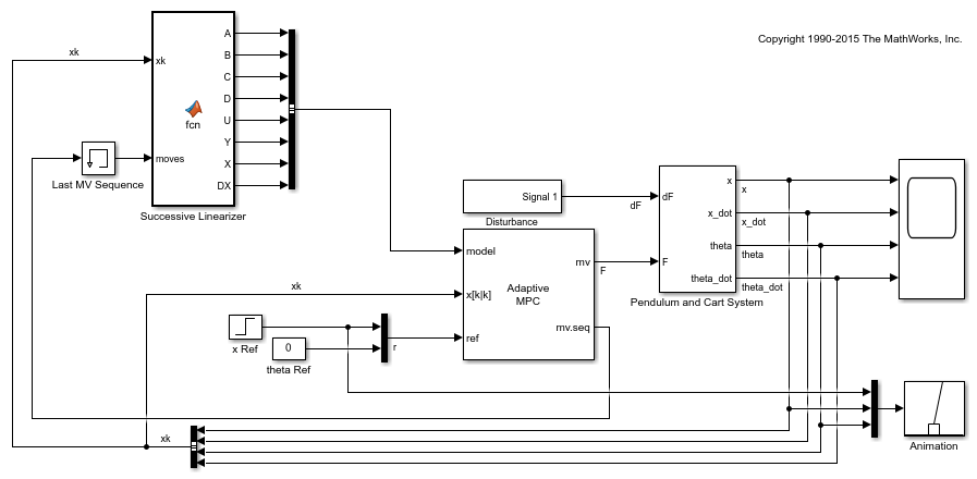
由于所有植物状态都是可测量的，因此它们在自适应MPC块中直接用作自定义估计状态。

While the cart position setpoint varies (step input), the pendulum angle setpoint is constant (0=upright position).

Linear Time-Varying Plant Models

在每个控制间隔中，LTV MPC从当前时间开始需要每个预测步骤的线性植物模型k到timek+p，，，，wherep是预测范围。

In this example, the cart and pendulum dynamic system is described by a first principle model. This model consists of a set of differential and algebraic equations (DAEs), defined in thependulumCT功能。有关更多详细信息，请参阅pendulumct.m。

这Successive LinearizerSimulink模型中的块金宝app在运行时生成LTV模型。在每个预测步骤中，块都会获得状态空间矩阵一种，，，，b，，，，C，，，，andd连续时间使用jacobian，然后将它们转换为离散的时间值。最初的植物状态x（k）是直接从植物中测量的。工厂输入序列包含MPC控制器在先前的控制间隔中产生的最佳移动。

自适应MPC设计

MPC控制器在其名义平衡工作点设计。

x0 = zeros(4,1); u0 = zeros(1,1);

使用ODE分析获得线性植物模型。

[~,~,A,B,C,D] = pendulumCT(x0, u0); plant = ss(A,B,C([1 3],:),D([1 3],:));% position and angle

为了控制不稳定的植物，控制器样品时间不能太大（干扰排斥不良）或太小（过多的计算负载）。同样，预测范围不能太长（植物不稳定模式会占主导地位）或太短（违反约束将是无法预料的）。在此示例中使用以下参数：

Ts = 0.01; PredictionHorizon = 60; ControlHorizon = 3;

创建MPC控制器。

mpcobj = mpc(c2d(plant,Ts),Ts,PredictionHorizon,ControlHorizon);

- >“ weights.manipulationvariables”属性为空。假设默认为0.00000。- >“ weights.manipulationVariablesrate”属性为空。假设默认为0.10000。- >“ weight.outputvariables”属性为空。假设默认为1.00000。对于输出（s）y1和零重量的输出y2

这re is a limitation on how much force can be applied to the cart, which is specified using hard constraints on the manipulated variableF。

mpcobj.mv.min = -100;mpcobj.mv.max = 100;

It is good practice to scale plant inputs and outputs before designing weights. In this case, since the range of the manipulated variable is greater than the range of the plant outputs by two orders of magnitude, scale the MV input by100。

mpcobj.MV.ScaleFactor = 100;

为了提高控制器的鲁棒性，请增加MV变化率的重量0。1到1。

mpcobj.Weights.MVRate = 1;

To achieve balanced performance, adjust the weights on the plant outputs. The first weight is associated with cart positionz，，，，and the second weight is associated with angleTheta。

mpcobj.Weights.OV = [0.6 1.2];

Use a gain as the output disturbance model for the pendulum angle. This represents rapid short-term variability.

setoutdist(mpcobj,'模型'，[0; tf（1）]）;

使用自定义状态估计，因为所有植物状态都是可衡量的。

setEstimator（mpcobj，'风俗');

闭环模拟

Validate the MPC design with a closed-loop simulation in Simulink.

open_system([mdlMPC'/Scope']); sim(mdlMPC)

- >“ model.noise”属性为空。假设每个测得的输出上都有白噪声。

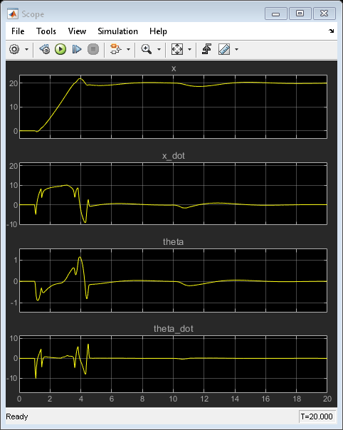
在非线性模拟中，所有控制目标都是成功实现的。

BDCLOSE（MDLMPC）;