Design PID Controller Using Simulated I/O Data
This example shows how to tune a PID controller for plants that cannot be linearized. You usePID Tunerto identify a plant for your model. Then tune the PID controller using the identified plant.
This example uses a buck converter model that requires Simscape™ Electrical™ software.
Buck Converter Model
Buck converters convert DC to DC. This model uses a switching power supply to convert a 30V DC supply into a regulated DC supply. The converter is modeled using MOSFETs rather than ideal switches to ensure that device on-resistances are correctly represented. The converter response from reference voltage to measured voltage includes the MOSFET switches. PID design requires a linear model of the system from the reference voltage to the measured voltage. However, because of the switches, automated linearization results in a zero system. In this example, usingPID Tuner, you identify a linear model of the system using simulation instead of linearization.
For more information on creating a buck converter model, seeBuck Converter(Simscape Electrical).
open_system('scdbuckconverter') sim('scdbuckconverter')

The model is configured with a reference voltage that switches from 15 to 25 Volts at 0.004 seconds and a load current that is active from 0.0025 to 0.005 seconds. The controller is initialized with default gains and results in overshoot and slow settling time.
open_system('scdbuckconverter/Scope 1') open_system('scdbuckconverter/Scope 2')


Simulate Model to Generate I/O Data
To open the PID Tuner, in theFeedback controllersubsystem, open thePID Controllerblock dialog, and clickTune.PID Tunerindicates that the model cannot be linearized and returned a zero system.

PID Tuner提供了几个选择when linearization fails. In thePlantdrop-down list, you can select one of the following methods:
Import- Import a linear model from the MATLAB workspace.
Re-linearize Closed Loop- Linearize the model at different simulation snapshot times.
Identify New Plant- Identify a plant model using measured data.
For this example, clickIdentify New Plantto open the Plant Identification tool. For plant identification, you must specify a finite value for the Simulink model stop time.

To open a tool that simulates the model to collect data for plant identification, on the植物鉴别tab, clickGet I/O Data > Simulate Data.

On theSimulate I/O Datatab, you simulate the plant seen by the controller. The software temporarily:
Removes the PID Controller block from the model.
Injects a signal where the output of the PID block used to be.
Measures the resulting signal where the input to the PID block used to be.
This data describes the response of the plant seen by the controller. ThePID Tuneruses this response data to estimate a linear plant model.
Configure the input signal as a step input with the following properties:
Sample Time (
 )= 5e-6 - Controller sample rate.
Offset (
 )= 0.51 - Output offset value that puts the converter in a state where the output voltage is near 15V and gives the operating point around which to tune the controller.
Onset Time (
 )= 0.003 - Delay to allow sufficient time for the converter to reach the 15V steady state before applying the step change.
Step Amplitude (
 )= 0.4 - Step size of the controller output (plant input) to apply to the model. This value is added to the offset valueso that the actual plant input steps from 0.51 to 0.91. The controller output (plant input) is limited to the range [0.01 0.95].


SelectShow Input Response,Show Offset Response, andShow Identification Data. Then, click theRun Simulation. The植物鉴别plot is updated.

The red curve is the offset response. The offset response is the plant response to a constant input of . The response shows that the model has some transients with a constant input, in particular:
The [0 0.001] second range where the converter reaches the 15V steady state. Recall that this signal is the control error signal and hence drops to zero as steady state is reached.
The [0.0025 0.004] second range where the converter reacts to the current load being applied while the reference voltage is maintained at 15V.
The 0.004 second point where the reference voltage signal is changed from 15V to 25V resulting in a larger control error signal.
The [0.005 0.006] second range where the converter reacts to the current load being removed.
The blue curve shows the complete plant response that contains the contributions from the initial transients (significant for times < 0.001 seconds), the response to the cyclic current load (time durations 0.0025 to 0.005 seconds), reference voltage change (at 0.004 seconds), and response to the step test signal (applied at time 0.003 seconds). In contrast, the red curve is the response to only the initial transients, reference voltage step, and cyclic current load.
The green curve is the data that will be used for plant identification. This curve is the change in response due to the step test signal, which is the difference between the blue (input response) and red (offset response) curves taking into account the negative feedback sign.
To use the measured data to identify a plant model, clickApply. Then, to return to plant identification, clickClose.
植物鉴别
PID Tuner标识一个工厂使用生成的数据模型by simulating the model. You tune the identified plant parameters so that the identified plant response, when provided the measured input, matches the measured output.

You can manually adjust the estimated model. Click and drag the plant curve and pole location (X) to adjust the identified plant response so that it matches the identification data as closely as possible.

To tune the identified plant using automated identification, clickAuto Estimate. The automated tuning response is not much better than the interactive tuning. The identified plant and identification data do not match well. Change the plant structure to get a better match.
In the Structure drop-down list, selectUnderdamped pair.
Click and drag the 2nd order envelope to match the identified data as closely as possible (almost critically damped).
ClickAuto Estimateto fine tune the plant model.


To designate the identified model as the current plant for controller tuning, ClickApply.PID Tunerthen automatically tunes a controller for the identified plant and updates theReference Trackingstep plot.
Controller Tuning
The PID Tuner automatically tunes a PID controller for the identified plant. The tuned controller response has about 5% overshoot and a settling time of around 0.0006 seconds. Click theReference Trackingstep plot to make it the current figure.

The controller output is the duty cycle for the PWM system and must be limited to [0.01 0.95]. To confirm that the controller output satisfies these bounds, create a controller effort plot. On thePID Tunertab, in theAdd Plotdrop-down list, underStep, clickController effort. Move the newly createdController effortplot to the second plot group.

In theController effortplot, the tuned response (solid line) shows a large control effort required at the start of the simulation. To achieve a settling time of about 0.0004 seconds and overshoot of 9%, adjust theResponse TimeandTransient Behaviorsliders. These adjustments reduce the maximum control effort to the acceptable range.

To update the Simulink block with the tuned controller values, clickUpdate Block.
To confirm the PID controller performance, simulate the Simulink model.

bdclose('scdbuckconverter')
See Also
Related Topics
- System Identification for PID Control(Simulink Control Design)
- Input/Output Data for Identification(Simulink Control Design)
- Interactively Estimate Plant from Measured or Simulated Response Data(Simulink Control Design)
- Choosing Identified Plant Structure(Simulink Control Design)
Select a Web Site
Choose a web site to get translated content where available and see local events and offers. Based on your location, we recommend that you select:.
Selectweb siteYou can also select a web site from the following list:
Americas
- América Latina(Español)
- Canada(English)
- United States(English)
Europe
- Belgium(English)
- Denmark(English)
- Deutschland(Deutsch)
- España(Español)
- Finland(English)
- France(Français)
- Ireland(English)
- Italia(Italiano)
- Luxembourg(English)
- Netherlands(English)
- Norway(English)
- Österreich(Deutsch)
- Portugal(English)
- Sweden(English)
- Switzerland
- United Kingdom(English)