Use State-Space Estimation to Reduce Model Order

Reduce the order of a Simulink^®model by linearizing the model and estimating a lower order model that retains model dynamics.

This example requires Simulink and theSimulink Control Design™toolbox.

Consider the Simulink modelidF14Model. Linearizing this model gives a ninth-order model. However, the dynamics of the model can be captured, without compromising the fit quality too much, using a lower-order model.

Obtain the linearized model.

load_system('idF14Model'); io = getlinio('idF14Model'); sys_lin = linearize('idF14Model',io);

sys_linis a ninth-order state-space model with two outputs and one input.

Simulate the step response of the linearized model, and use the data to create aniddataobject.

Ts = 0.0444; t = (0:Ts:4.44)'; y = step(sys_lin,t); data = iddata([zeros(20,2);y],[zeros(20,1); ones(101,1)],Ts);

datais aniddataobject that encapsulates the step response ofsys_lin.

Compare the data to the model linearization.

compare(data,sys_lin);

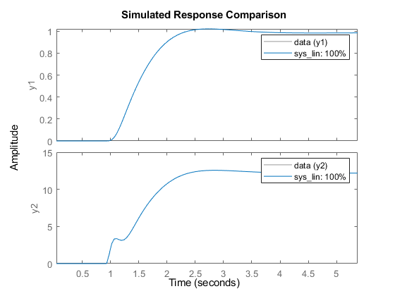
Because the data was obtained by simulating the linearized model, there is a complete match between the data and model linearization response.

Identify a state-space model with a reduced order that adequately fits the data.

Determine an optimal model order.

nx = 1:9; sys1 = ssest(data,nx,'DisturbanceModel','none');

A plot showing the Hankel singular values (SVD) for models of the orders specified bynxappears.

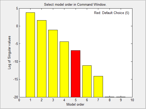
States with relatively small Hankel singular values can be safely discarded. The plot suggests using a fifth-order model.

At the MATLAB^®命令提示符,选择模型为美国东部时间imated state-space model. Specify the model order as5, or pressEnterto use the default order value.

Compare the data to the estimated model.

compare(data,sys1);

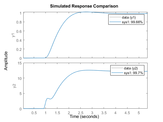
The plot displays the fit percentages for the twosys1outputs. The four-state reduction in model order results in a relatively small reduction in fit percentage.

Examine the stopping condition for the search algorithm.

sys1.Report.Termination.WhyStop

ans = 'Maximum number of iterations reached.'

Create an estimation options set. Specify the'lm'search method. Increase the maximum number of search iterations to 50 from the default maximum of 20.

opt = ssestOptions('SearchMethod','lm'); opt.SearchOptions.MaxIterations = 50; opt.Display ='on';

识别使用估计的状态空间模型option set andsys1as the estimation initialization model.

sys2 = ssest(data,sys1,opt);

Compare the response of the linearized and the estimated models.

compare(data,sys_lin,sys2);

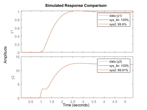
The updated option set results in better fit percentages forsys2.

See Also

linearize(Simulink Control Design)|getlinio(Simulink Control Design)