Analyzing Simple ADC with Impairments
此示例显示了如何使用零级保持块作为采样器实现基本ADC。这种简单的ADC强调了在类似物到数字转换器中引入的一些典型障碍,例如光圈抖动,非线性,量化和饱和度。此示例显示了如何使用Spectrum Analyzer块和来自混合信号阻滞™的ADC AC测量块来测量此类损伤的效果。为了更好地近似现实世界的性能,您可以单独实现模型中的损害。
模型='MSADCImpairments'; open_system(model)
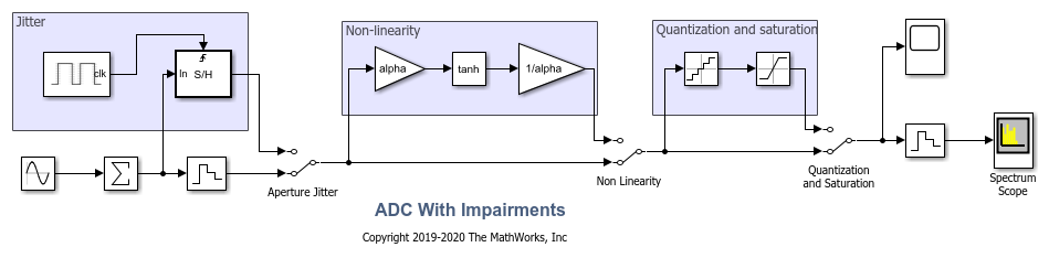
To observe the behavior of an ideal ADC, bypass the impairments using the switches. Set the Sine Wave source to generate two tones as an input signal.
set_param([模型'/Aperture Jitter'],'sw','1');set_param([模型'/Non Linearity'],'sw','0');set_param([模型'/Quantization and Saturation'],'sw','0');set_param([模型'/Sine Wave'],'Frequency','2*pi*[47 53]*1e6');
Simulate the model and observe the expected clean output spectrum of the ADC.
sim(model);

Effect of Aperture Jitter
Set the first switch to the down position. The Variable Delay block delays the signal sample-by-sample by the amount on itstdinput. The Noise Source block generates a uniform random variable, which is low-pass filtered by the Shape the jitter noise spectrum block before it arrives at thetd输入变量延迟。使用形状均匀的噪声分布来表示抖动。请注意,在此模型中,ADC的时钟是在理想的零级保持块中指定的,并且等于1/fs,其中FS是模型初始化回调中定义的MATLAB®变量,并等于1.024GHz。
set_param([模型'/Aperture Jitter'],'sw','0');
As expected, the spectrum degrades because of the presence of the jitter.
sim(model);

Effect of Nonlinearity
Set the second switch to the up position. This enables the ADC nonlinearity. A scaled hyperbolic tangent function provides nonlinearity. Its scale factor,alpha,确定s the amount of nonlinearity the tanh applies to the signal. By default,alphais0.01.
set_param([模型'/Non Linearity'],'sw','1');
由于非线性的产生,因此由于非线性而降低了频谱。
sim(model);

Effect of Quantization and Saturation
Set the third switch to the up position enabling the ADC quantization and hard saturation.
set_param([模型'/Quantization and Saturation'],'sw','1');
The spectrum degrades because of the quantization effects. The noise floor raises as seen in the spectrum.
sim(model);

ADC交流测量
使用混合信号阻滞™中的ADC AC测量块来测量ADC的噪声性能,并计算有效数量(ENOB)。
Use single sinusoidal tone as input to the ADC to measure other metrics.
bdclose(模型);模型='msadcimpairments_ac'; open_system(model);

Ftest = 33/round(2*pi*2^8)*Fs; set_param([model'/Sine Wave'],'Frequency','2*pi*ftest');scopecfg = get_param([模型'/Spectrum Scope'],'ScopeConfiguration');scopecfg.DistortionMeasurements.Algorithm ='Harmonic'; scopecfg.FFTLength ='512'; scopecfg.WindowLength ='512'; sim(model);

The Aperture Jitter Measurement block from Mixed-Signal Blockset™ measures the average jitter introduced on the signal to be approximately equal to1ps.
Additionally, use the spectrum analyzer to measure:
Output Third Order Intercept Point (OIP3)
Signal to Noise Ratio (SNR)
Total Harmonic Distortion (THD)
Increase the factoralphato increase the nonlinearity of the ADC and make the effects of nonlinearity more evident on top of the noise floor. This is just for demonstration purposes.
alpha = 0.8;
Use a two tone test signal as input to the ADC for the intermodulation measurements.
set_param([模型'/Sine Wave'],'Frequency','2*pi*[50E6 75E6]');
To enable distortion measurements in the spectrum analyzer, click onDistortion Measurementas in the figure below and selectIntermodulationasDistortiontype.
scopecfg.DistortionMeasurements.Algorithm ='Intermodulation'; scopecfg.FFTLength ='4096'; scopecfg.WindowLength ='4096'; sim(model);

The scope allows for the measurement of the third order products adjacent to the input signals, and determines the output referred third order intercept point.
See Also
Sampling Clock Source|Aperture Jitter Measurement|ADC AC测量
相关话题
You can also select a web site from the following list:
Americas
- AméricaLatina(Español)
- Canada(English)
- United States(English)
欧洲
- Belgium(English)
- 丹麦(English)
- Deutschland(德意志)
- España(Español)
- Finland(English)
- 法国(Français)
- 爱尔兰(English)
- Italia(Italiano)
- Luxembourg(English)
- Netherlands(English)
- 挪威(English)
- Österreich(德意志)
- Portugal(English)
- Sweden(English)
- Switzerland
- United Kingdom(English)