Introduction

在线性预测的情况下，目的是基于过去样本的线性组合来确定可以最佳地预测自回归过程的未来样本的FIR滤波器。实际自回归信号与预测信号之间的差异称为预测误差。理想情况下，此错误是白噪声。

For the case of autoregressive modeling, the intention is to determine an all-pole IIR filter, that when excited with white noise produces a signal with the same statistics as the autoregressive process that we are trying to model.

使用具有白色噪声的全极滤波器产生AR信号作为输入

在这里，我们使用LPC函数和FIR过滤器即可借出我们将使用的参数来创建自动增加信号我们将使用。FiR1和LPC的使用并不重要。例如，我们可以用东西替换为简单的东西[1/2 1/3 1/4 1/5 1/6 1/7 1/8]和p0，其中有类似于1E-6的东西。但这种过滤器的形状是更好的，所以我们使用它。

b = fir1(1024, .5); [d,p0] = lpc(b,7);

To generate the autoregressive signal, we will excite an all-pole filter with white Gaussian noise of variance p0. Notice that to get variance p0, we must use SQRT(p0) as the 'gain' term in the noise generator.

RNG（0，'twister'）;% Allow reproduction of exact experimentU = SQRT（P0）* RANDN（8192,1）;％白色高斯噪声具有方差P0

We now use the white Gaussian noise signal and the all-pole filter to generate an AR signal.

x = filter(1,d,u);

Find AR Model from Signal using the Yule-Walker Method

Solving the Yule-Walker equations, we can determine the parameters for an all-pole filter that when excited with white noise will produce an AR signal whose statistics match those of the given signal, x. Once again, this is called autoregressive modeling. In order to solve the Yule-Walker equations, it is necessary to estimate the autocorrelation function of x. The Levinson algorithm is used then to solve the Yule-Walker equations in an efficient manner. The function ARYULE does all this for us.

[d1，p1] = aryule（x，7）;

使用AR信号进行比较AR模型

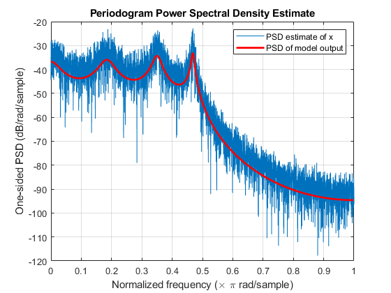
我们现在想计算我们刚刚用于模拟AR信号X的全极过滤器的频率响应。众所周知，当滤波器激发与白色高斯噪声激发时，通过白色高斯噪声激发滤波器的功率谱密度由其频率响应的幅度平方乘以白噪声输入的方差。计算该输出功率谱密度的一种方法是使用Freqz如下：

[H1，W1] = Freqz（SQRT（P1），D1）;

为了了解我们对自回归信号X的建模有何建模，我们覆盖了使用FREQZ计算的模型输出的功率谱密度，使用X的功率谱密度估计，使用循序量目率计算。请注意，期间焦点由2 * PI缩放，并且是片面的。我们需要调整此项以便比较。

句号（x）持有onhp = plot(w1/pi,20*log10(2*abs(H1)/(2*pi)),'r'）;% Scale to make one-sided PSDhp.LineWidth = 2; xlabel('归一化频率（\ Times \ Pi Rad / Sample）'的）ylabel('One-sided PSD (dB/rad/sample)'） 传奇（'PSD估计x'那'PSD of model output'的）

使用LPC执行线性预测

We now turn to the linear prediction problem. Here we try to determine an FIR prediction filter. We use LPC to do so, but the result from LPC requires a little interpretation. LPC returns the coefficients of the entire whitening filter A(z), this filter takes as input the autoregressive signal x and returns as output the prediction error. However, A(z) has the prediction filter embedded in it, in the form B(z) = 1- A(z), where B(z) is the prediction filter. Note that the coefficients and error variance computed with LPC are essentially the same as those computed with ARYULE, but their interpretation is different.

[D2，P2] = LPC（x，7）;[d1'，d2。']

ANS =.8×21.0000 1.0000 -3.5245 -3.5245 6.9470 6.9470 -9.2899 -9.2899 8.9224 8.9224 8.9224 -6.1349 -6.1349 2.8299 2.8299 -0.6997 -0.6997

We now extract B(z) from A(z) as described above to use the FIR linear predictor filter to obtain an estimate of future values of the autoregressive signal based on linear combinations of past values.

xh =滤波器（-d2（2：端），1，x）;

比较实际和预测的信号

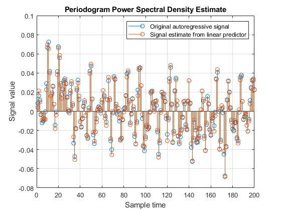
To get a feeling for what we have done with a 7-tap FIR prediction filter, we plot (200 samples) of the original autoregressive signal along with the signal estimate resulting from the linear predictor keeping in mind the one-sample delay in the prediction filter.

CLA茎（[x（2：末端），XH（1：end-1）]）XLabel（'Sample time'的）ylabel('信号值'） 传奇（'原始自回归信号'那'从线性预测器的信号估计'的）axis([0 200 -0.08 0.1])

Compare Prediction Errors

预测误差功率（方差）作为来自LPC的第二输出返回。其值（理论上）是与在AR建模问题中驱动全极滤波器的白噪声的方差相同（P1）。估计这种方差的另一种方法是来自预测错误本身：

p3 = norm(x(2:end)-xh(1:end-1),2)^2/(length(x)-1);

所有以下值都是同样的。差异是由于本文的各种计算和近似误差。

[p0 p1 p2 p3]

ANS =.1×4.10.-5×0.5127 0.5305 0.5305 0.5068