使用ClassificationEnsemble预测块预测类标签
此示例演示如何使用最佳超参数训练集合模型,然后使用分类编码预测Simulink®中标签预测的块。该块接受一个观测值(预测器金宝app数据),并使用经过训练的分类集成模型返回观测值的预测类标签和类分数。
具有最优超参数的列车分类模型
加载Creditrating_Historical.数据集。此数据集包含客户ID及其财务比率、行业标签和信用评级。确定样本大小。
tbl =可读取的(“信用评级历史数据”); n=努美尔(待定)
n=31456
显示表的前三行。
头部(待定,3)
ans =3×8表ID WC_TA RE_TA EBIT_TA MVE_BVTD S_TA行业评级 _____ _____ _____ _______ ________ _____ ________ ______ 62394 0.013 0.104 0.036 0.447 0.142 3{“BB”}48608 0.232 0.335 0.062 1.969 0.281 8 {A} 42444 0.311 0.367 0.074 1.935 0.366 1 {A}
资源描述。行业是行业标签的分类变量。为ClassificationnSemble Predict块训练模型时,必须使用杜姆瓦尔在模型中包含分类预测器的功能。你不能使用“分类预测因素”名称-值参数。创建虚拟变量资源描述。行业.
d=dummyvar(待定行业);
杜姆瓦尔的每个类别创建虚拟变量资源描述。行业. 确定中的类别数资源描述。行业和中虚拟变量的数量D.
独特(待定行业)'
ans =1×12.1 2 3 4 5 6 7 8 9 10 11 12
大小(d)
ans =1×23932年12
为预测变量创建数字矩阵,为响应变量创建单元格数组。
X = [table2array(tbl(:,2:6)) d];Y = tbl.Rating;
X是一个数字矩阵,包含17个变量:五个财务比率和行业标签的12个虚拟变量。X不使用tbl.ID因为变量没有有助于预测信用评级。Y是字符向量的单元格数组,其中包含相应的信用评级。
假设您按顺序接收了数据,并且已经有了前3000个观测值,但还没有收到最后932个。将数据划分为当前和未来的样本。
prsntX=X(1:3000,:);prsntY=Y(1:3000);ftrX=X(3001:end,:);ftrY=Y(3001:end);
使用所有目前可用的数据列车prsntX和prsntY这些选项:
具体说明
“优化超参数”像“自动”用最佳的QuandeParameter培训合奏。这个“自动”选项可为以下项找到最佳值:“方法”,“NumLearningCycles”,“LearnRate”(适用方法)的菲特森布尔和“MinLeafSize”树学习者。对于再现性,设置随机种子并使用
“expected-improvement-plus”采集功能。此外,对于随机森林算法的再现性,请指定“可复制”像真正的适合树木学习者。属性指定类的顺序
“类名”名称-值参数。的输出值分数ClassificationnSemble Predict块的端口具有相同的顺序。
rng (“默认”)t=模板树(“可复制”,真的);ensmdl = fitcensemble(prsntx,prsnty,...“类名”, {“AAA”“AA”“A”'BBB'“BB”“B”“CCC”},...“优化超参数”,“自动”,“学习者”,t,...“HyperparameterOptimizationOptions”,...结构(“AcquisitionFunctionName”,“expected-improvement-plus”))
| ===================================================================================================================================|磨练|eval |目标|目标|Bestsofar |Bestsofar |方法|numlearningc- | LearnRate | MinLeafSize | | | result | | runtime | (observed) | (estim.) | | ycles | | | |===================================================================================================================================| | 1 | Best | 0.51133 | 13.652 | 0.51133 | 0.51133 | AdaBoostM2 | 429 | 0.082478 | 871 | | 2 | Best | 0.26133 | 18.827 | 0.26133 | 0.27463 | AdaBoostM2 | 492 | 0.19957 | 4 | | 3 | Accept | 0.85133 | 0.76925 | 0.26133 | 0.28421 | RUSBoost | 10 | 0.34528 | 1179 | | 4 | Accept | 0.263 | 0.61254 | 0.26133 | 0.26124 | AdaBoostM2 | 13 | 0.27107 | 10 | | 5 | Best | 0.26 | 0.9413 | 0.26 | 0.26003 | Bag | 10 | - | 1 | | 6 | Accept | 0.28933 | 1.7101 | 0.26 | 0.2602 | Bag | 36 | - | 101 | | 7 | Best | 0.25667 | 1.3583 | 0.25667 | 0.25726 | AdaBoostM2 | 33 | 0.99501 | 11 | | 8 | Best | 0.244 | 28.725 | 0.244 | 0.24406 | Bag | 460 | - | 7 | | 9 | Accept | 0.246 | 4.19 | 0.244 | 0.24435 | Bag | 60 | - | 4 | | 10 | Accept | 0.25533 | 1.3969 | 0.244 | 0.24437 | AdaBoostM2 | 33 | 0.99516 | 1 | | 11 | Accept | 0.25733 | 1.5294 | 0.244 | 0.2442 | Bag | 25 | - | 8 | | 12 | Accept | 0.74267 | 16.444 | 0.244 | 0.24995 | Bag | 488 | - | 1494 | | 13 | Accept | 0.28567 | 7.9382 | 0.244 | 0.24624 | RUSBoost | 158 | 0.0010063 | 1 | | 14 | Accept | 0.257 | 23.416 | 0.244 | 0.24559 | Bag | 491 | - | 31 | | 15 | Accept | 0.28433 | 0.71501 | 0.244 | 0.24557 | RUSBoost | 12 | 0.48085 | 6 | | 16 | Accept | 0.267 | 17.82 | 0.244 | 0.2456 | AdaBoostM2 | 484 | 0.0028818 | 43 | | 17 | Accept | 0.24667 | 33.219 | 0.244 | 0.24601 | Bag | 488 | - | 3 | | 18 | Best | 0.244 | 34.953 | 0.244 | 0.2454 | Bag | 498 | - | 3 | | 19 | Accept | 0.24467 | 31.568 | 0.244 | 0.24489 | Bag | 473 | - | 3 | | 20 | Accept | 0.259 | 19.187 | 0.244 | 0.24488 | AdaBoostM2 | 497 | 0.67001 | 19 | |===================================================================================================================================| | Iter | Eval | Objective | Objective | BestSoFar | BestSoFar | Method | NumLearningC-| LearnRate | MinLeafSize | | | result | | runtime | (observed) | (estim.) | | ycles | | | |===================================================================================================================================| | 21 | Accept | 0.27733 | 19.735 | 0.244 | 0.24468 | RUSBoost | 386 | 0.91461 | 2 | | 22 | Accept | 0.245 | 32.172 | 0.244 | 0.2441 | Bag | 482 | - | 4 | | 23 | Accept | 0.244 | 33.117 | 0.244 | 0.24388 | Bag | 497 | - | 4 | | 24 | Accept | 0.245 | 34.32 | 0.244 | 0.24406 | Bag | 497 | - | 4 | | 25 | Best | 0.243 | 33.134 | 0.243 | 0.24394 | Bag | 499 | - | 5 | | 26 | Accept | 0.25733 | 0.55541 | 0.243 | 0.24371 | AdaBoostM2 | 12 | 0.87848 | 53 | | 27 | Accept | 0.263 | 0.52438 | 0.243 | 0.24371 | AdaBoostM2 | 11 | 0.6978 | 2 | | 28 | Accept | 0.24367 | 31.167 | 0.243 | 0.24344 | Bag | 484 | - | 5 | | 29 | Accept | 0.292 | 19.748 | 0.243 | 0.24342 | AdaBoostM2 | 497 | 0.0010201 | 1 | | 30 | Accept | 0.292 | 0.7854 | 0.243 | 0.24342 | RUSBoost | 13 | 0.0012334 | 3 |

__________________________________________________________优化完成。MaxObjectiveEvaluation达到了30。总功能评估:30总运行时间:488.5833秒总目标功能评估时间:464.2275最佳观察可行点:方法NumLearningCycles LearnrRate Minleaf Size uuuuuuuuuuuuuuuuuuuuuuuuuuuuuuuuuuuuuuuuuuuuuuuuuuuuuuuuuuuuuuuuuuuuuuuuuuuuuuuuuuuuuuuuuuuuuuuuuuuuuuuuuuuuuuuuuuuuuuuuuuuuuuuuuuuuuuuuuuuuuuuuuuuuuuuuuuuu功能评估时间=33.1343最佳估计可行点(根据模型):方法NumLearningCycles LearnRate MinLeaf Size\uuuuuuuuuuuuuuuuuuuuuuuuuuuuuuuuuuuuuuuuuuuuuuuuuuuuuuuuuuuuuuuuuuuuuuuuuuu5估计目标函数值=0.24342估计功能评估时间=32.1002
ensMdl = ClassificationBaggedEnsemble ResponseName:‘Y’CategoricalPredictors:[]类名:{“AAA”“AA”的一个“BBB的“BB”“B”“CCC”}ScoreTransform:“没有一个”NumObservations: 3000 HyperparameterOptimizationResults:[1×1 BayesianOptimization] NumTrained: 499方法:“袋子”LearnerNames:{‘树’}ReasonForTermination:“在完成要求的培训周期数后正常终止。”userobsforlearner: [3000×499 logical]属性,方法
菲特森布尔返回一个ClassificationBaggedEnsemble对象,因为该函数找到随机森林算法(“包”)作为最佳方法。
创建Simul金宝appink模型
这个例子提供了Simulink模型金宝appSLEXCreditingClassificationnSemblePredictExample.slx,其中包括分类编码预测块。您可以打开Simulink模型或创金宝app建本节所述的新模型。
打开Simulin金宝appk模型SLEXCreditingClassificationnSemblePredictExample.slx.
SimMdlName ='SlexcreditrationClassificationsemblePredictExample';open_system (SimMdlName)

这个预处理回调函数的SLEXCreditingClassificationnSemblePredictExample包括加载样本数据、使用最优超参数训练模型以及为Simulink模型创建输入信号的代码。金宝app如果打开Simulink模型,软金宝app件就会运行代码预处理加载Simulink模型之前。要查看回金宝app调函数,请在安装程序关于建模选项卡,单击模型设置选择模型属性.然后,在回调选项卡中,选择预处理的回调函数模型的回调窗格。
要创建新的Simulink模型,金宝app请打开空白模型模板并添加ClassificationnSemble预测块。添加输入和输出块并将它们连接到ClassificationnSemble预测块。
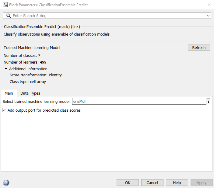
双击分类uslemble预测块以打开块参数对话框。指定选择培训的机器学习模型参数为ensMdl,它是包含训练模型的工作空间变量的名称。单击刷新按钮。对话框显示用于训练模型的选项ensMdl在下面训练机器学习模型.选择添加预测类分数的输出端口复选框以添加第二个输出端口分数.
分类型预测块期望包含17个预测值值的观察。双击Inport块,并设置端口尺寸到17号信号属性选项卡。
以结构数组的形式为Simulink模型创建一个输入信号。金宝app结构数组必须包含以下字段:
时间-观察值进入模型的时间点。在本例中,持续时间包括从0到931的整数。方向必须与预测数据中的观察值相对应。因此,在本例中,时间必须是列向量。信号-描述输入数据并包含字段的1×1结构数组值和方面,在那里值是预测数据的矩阵,以及方面为预测变量的数量。
为将来的示例创建适当的结构数组。
CreditRatingInput.time =(0:931)';CreditRatingInput.Signals(1).values = ftrx;CreditRatingInput.Signals(1).dimensions =尺寸(ftrx,2);
从工作区导入信号数据:
打开“配置参数”对话框。在建模选项卡,单击模型设置.
在数据导入/导出窗格中,选择输入选中复选框并输入
信贷投入在相邻的文本框中。在解算器窗格,在下面模拟时间设置停止时间到
creditRatingInput.time(结束)在下面解算器的选择设置类型到固定步长,并设置解算器到离散(无连续状态).
有关详细信息,请参见用于仿真的负载信号数据(金宝appSimulink).
模拟模型。
sim (SimMdlName);
当输入块检测到一个观测值时,它将观测值引导到ClassificationnSemble Predict块。你可以使用模拟数据检查器(金宝appSimulink)查看输出端口块的记录数据。
另见
相关的话题
您还可以从以下列表中选择一个网站: