Wavelet Interval-Dependent Denoising

Open Live Script

The example shows how to denoise a signal using interval-dependent thresholds.

Wavelet GUI tools provide an accurate denoising process by allowing us to fine tune the parameters required to denoise a signal. Then, we can save the denoised signal, the wavelet decomposition and all denoising parameters.

It can be tedious and sometimes impossible to treat many signals using the same denoising settings. A batch mode, using the command line, can be much more efficient. This example shows how to work at the command line to simplify and solve this problem.

In this example, we perform six trials to denoise the electrical signalnelecusing these procedures:

Using one interval with the minimum threshold value: 4.5
Using one interval with the maximum threshold value: 19.5
Manually selecting three intervals and three thresholds, and using thewthreshfunction to threshold the coefficients.
Using theutthrset_cmdfunction to automatically find the intervals and the thresholds.
Using thecmddenoisefunction to perform all the processes automatically.
Using thecmddenoisefunction with additional parameters.

Denoising Using a Single Interval

Load the electrical consumption signalnelec.

loadnelec.matsig = nelec;

Now we use the discrete wavelet analysis atlevel 5with thesym4wavelet. We set the thresholding type to's'(soft).

wname ='sym4'; level = 5; sorh ='s';

Denoise the signal using the functionwdencmpwith the threshold set at4.5, which is the minimum value provided by the GUI tools.

thr = 4.5; [sigden_1,~,~,perf0,perfl2] = wdencmp('gbl',sig,wname,level,thr,sorh,1); res = sig-sigden_1; subplot(3,1,1) plot(sig,'r') axistighttitle('Original Signal') subplot(3,1,2) plot(sigden_1,'b') axistighttitle('Denoised Signal') subplot(3,1,3) plot(res,'k') axistighttitle('Residual')

Figure contains 3 axes objects. Axes object 1 with title Original Signal contains an object of type line. Axes object 2 with title Denoised Signal contains an object of type line. Axes object 3 with title Residual contains an object of type line.

perf0,perfl2

perf0 = 66.6995

perfl2 = 99.9756

The obtained result is not good. The denoising is very efficient at the beginning and end of the signal, but between 100 and 1100 the noise is not removed. Note that theperf0value gives the percentage of coefficients set to zero and theperfl2value gives the percentage of preserved energy.

Now, we denoise the signal with the maximum value provided by the GUI tools for the threshold,19.5

thr = 19.5; [sigden_2,cxd,lxd,perf0,perfl2] = wdencmp('gbl',sig,wname,level,thr,sorh,1); res = sig-sigden_2; subplot(3,1,1) plot(sig,'r') axistighttitle('Original Signal') subplot(3,1,2) plot(sigden_2,'b') axistighttitle('Denoised Signal') subplot(3,1,3) plot(res,'k') axistighttitle('Residual')

perf0,perfl2

perf0 = 94.7860

perfl2 = 99.9564

The denoised signal is very smooth. It seems quite good, but if we look at the residual after position 1100, we can see that the variance of the underlying noise is not constant. Some components of the signal have likely remained in the residual, such as, near the position 1300 and between positions 1900 and 2000.

Denoising Using the Interval Dependent Thresholds (IDT)

Now we will use an interval-dependent thresholding, as in the denoising GUI tools.

Perform a discrete wavelet analysis of the signal.

[coefs,longs] = wavedec(sig,level,wname);

Using the GUI tools to perform interval-dependent thresholding for the signalnelec, and setting the number of intervals at three, we get the content of thedenPARvariable, which can be interpreted as follows:

I1 = [1 94]with a thresholdthr1 = 5.9
I2 = [94 1110]with a thresholdthr2 = 19.5
I3 = [1110 2000]with a thresholdthr3 = 4.5

Define the interval-dependent thresholds.

denPAR = {[1 94 5.9 ; 94 1110 19.5 ; 1110 2000 4.5]}; thrParams = cell(1,level); thrParams(:) = denPAR;

Show the wavelet coefficients of the signal and the interval-dependent threshold for each level of the discrete analysis.

% Replicate the coefficientscfs_beg = wrepcoef(coefs,longs);% Display the coefficients of the decompositionfigure subplot(6,1,1) plot(sig,'r') axistighttitle('Original Signal and Detail Coefficients from 1 to 5') ylabel('S','Rotation',0)fork = 1:level subplot(6,1,k+1) plot(cfs_beg(k,:),'Color',[0.5 0.8 0.5]) ylabel(['D'int2str(k)],'Rotation',0) axistightholdonmaxi = max(abs(cfs_beg(k,:))); holdonpar = thrParams{k}; plotPar = {'Color','m','LineStyle','-.'};forj = 1:size(par,1)-1 plot([par(j,2),par(j,2)],[-maxi maxi],plotPar{:})endforj = 1:size(par,1) plot([par(j,1),par(j,2)],[par(j,3) par(j,3)],plotPar{:}) plot([par(j,1),par(j,2)],-[par(j,3) par(j,3)],plotPar{:})endylim([-maxi*1.05 maxi*1.05])%hold offendsubplot(6,1,level+1) xlabel('Time or Space')

图包含6轴对象。坐标轴对象1title Original Signal and Detail Coefficients from 1 to 5 contains an object of type line. Axes object 2 contains 9 objects of type line. Axes object 3 contains 9 objects of type line. Axes object 4 contains 9 objects of type line. Axes object 5 contains 9 objects of type line. Axes object 6 contains 9 objects of type line.

For each levelk, the variablethrParams{k}contains the intervals and the corresponding thresholds for the denoising procedure.

Threshold the wavelet coefficients level-by-level, and interval-by- interval, using the values contained in thethrParamsvariable.

Using the functionwthresh, we threshold the wavelet coefficients values between the horizontal lines by replacing them with zeros, while other values are either reduced ifsorh = 's'or remain unchanged ifsorh = 'h'.

first = cumsum(longs)+1; first = first(end-2:-1:1); tmp = longs(end-1:-1:2); last = first+tmp-1;fork = 1:level thr_par = thrParams{k};if~isempty(thr_par) cfs = coefs(first(k):last(k)); nbCFS = longs(end-k); NB_int = size(thr_par,1); x = [thr_par(:,1) ; thr_par(NB_int,2)]; alf = (nbCFS-1)/(x(end)-x(1)); bet = 1 - alf*x(1); x = round(alf*x+bet); x(x<1) = 1; x(x>nbCFS) = nbCFS; thr = thr_par(:,3);forj = 1:NB_intifj == 1 d_beg = 0;elsed_beg = 1;endj_beg = x(j)+ d_beg; j_end = x(j+1); j_ind = (j_beg:j_end); cfs(j_ind) = wthresh(cfs(j_ind),sorh,thr(j));endcoefs(first(k):last(k)) = cfs;endend

Show the thresholded wavelet coefficients of the signal.

% Replicate the coefficients.cfs_beg = wrepcoef(coefs,longs);% Display the decomposition coefficients.figure subplot(6,1,1) plot(sig,'r') axistighttitle('Original Signal and Detail Coefficients from 1 to 5') ylabel('S','Rotation',0)fork = 1:level subplot(6,1,k+1) plot(cfs_beg(k,:),'Color',[0.5 0.8 0.5]) ylabel(['D'int2str(k)],'Rotation',0) axistightholdonmaxi = max(abs(cfs_beg(k,:)));%hold onpar = thrParams{k}; plotPar = {'Color','m','LineStyle','-.'};forj = 1:size(par,1)-1 plot([par(j,2),par(j,2)],[-maxi maxi],plotPar{:})endforj = 1:size(par,1) plot([par(j,1),par(j,2)], [par(j,3) par(j,3)],plotPar{:}) plot([par(j,1),par(j,2)],-[par(j,3) par(j,3)],plotPar{:})endylim([-maxi*1.05 maxi*1.05]) holdoffendsubplot(6,1,level+1) xlabel('Time or Space')

Reconstruct the denoised signal.

sigden = waverec(coefs,longs,wname); res = sig - sigden;

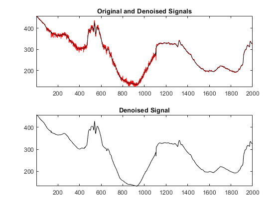
Display the original, denoised, and residual signals.

figure subplot(3,1,1) plot(sig,'r') holdonplot(sigden,'b') axistighttitle(原始和去噪信号) subplot(3,1,2) plot(sigden,'b') axistighttitle('Denoised Signal') subplot(3,1,3) plot(res,'k') axistighttitle('Residual')

Figure contains 3 axes objects. Axes object 1 with title Original and Denoised Signals contains 2 objects of type line. Axes object 2 with title Denoised Signal contains an object of type line. Axes object 3 with title Residual contains an object of type line.

Compare the three denoised versions of the signal.

figure plot(sigden_1,'g') holdonplot(sigden_2,'r') plot(sigden,'k') axistightholdofflegend('Denoised Min','Denoised Max','Denoised IDT','Location','North')

Figure contains an axes object. The axes object contains 3 objects of type line. These objects represent Denoised Min, Denoised Max, Denoised IDT.

Looking at the first half of the signals, it is clear that denoising using the minimum value of the threshold is not good. Now, we zoom on the end of the signal for more details.

xlim([1200 2000]) ylim([180 350])

Figure contains an axes object. The axes object contains 3 objects of type line. These objects represent Denoised Min, Denoised Max, Denoised IDT.

We can see that when the maximum threshold value is used, the denoised signal is smoothed too much and information is lost.

The best result is given by using the threshold based on the interval- dependent thresholding method, as we will show now.

Automatic Computation of Interval-Dependent Thresholds

Instead of manually setting the intervals and the thresholds for each level, we can use the functionutthrset_cmdto automatically compute the intervals and the thresholds for each interval. Then, we complete the procedure by applying the thresholds, reconstructing, and displaying the signal.

% Wavelet Analysis.[coefs,longs] = wavedec(sig,level,wname); siz = size(coefs); thrParams = utthrset_cmd(coefs,longs); first = cumsum(longs)+1; first = first(end-2:-1:1); tmp = longs(end-1:-1:2); last = first+tmp-1;fork = 1:level thr_par = thrParams{k};if~isempty(thr_par) cfs = coefs(first(k):last(k)); nbCFS = longs(end-k); NB_int = size(thr_par,1); x = [thr_par(:,1) ; thr_par(NB_int,2)]; alf = (nbCFS-1)/(x(end)-x(1)); bet = 1 - alf*x(1); x = round(alf*x+bet); x(x<1) = 1; x(x>nbCFS) = nbCFS; thr = thr_par(:,3);forj = 1:NB_intifj==1 d_beg = 0;elsed_beg = 1;endj_beg = x(j)+d_beg; j_end = x(j+1); j_ind = (j_beg:j_end); cfs(j_ind) = wthresh(cfs(j_ind),sorh,thr(j));endcoefs(first(k):last(k)) = cfs;endendsigden = waverec(coefs,longs,wname); figure subplot(2,1,1) plot(sig,'r') axistightholdonplot(sigden,'k') title(原始和去噪信号) subplot(2,1,2) plot(sigden,'k') axistightholdofftitle('Denoised Signal')

Figure contains 2 axes objects. Axes object 1 with title Original and Denoised Signals contains 2 objects of type line. Axes object 2 with title Denoised Signal contains an object of type line.

Automatic Interval-Dependent Denoising

In command-line mode, we can use the functioncmddenoiseto automatically compute the denoised signal and coefficients based on the interval-dependent denoising method. This method performs the whole process of denoising using only this one function, which includes all the steps described earlier in this example.

[sigden,~,thrParams] = cmddenoise(sig,wname,level); thrParams{1}% Denoising parameters for level 1.

ans =2×310³× 0.0010 1.1100 0.0176 1.1100 2.0000 0.0045

The automatic procedure finds two intervals for denoising:

I1 = [1 1110]with a thresholdthr1 = 17.6
I2 = [1110 2000]with a thresholdthr2 = 4.5.

我们可以显示de的结果noising and see that the result is fine.

figure subplot(2,1,1) plot(sig,'r') axistightholdonplot(sigden,'k') title(原始和去噪信号) holdoffsubplot(2,1,2) plot(sigden,'k') axistighttitle('Denoised Signal')

Figure contains 2 axes objects. Axes object 1 with title Original and Denoised Signals contains 2 objects of type line. Axes object 2 with title Denoised Signal contains an object of type line.

Advanced Automatic Interval-Dependent Denoising

Now, we look at a more complete example of the automatic denoising.

Rather than using the default values for the input parameters, we can specify them when calling the function. Here, the type of threshold is chosen ass(soft) and the number of intervals is set at 3.

loadnelec.mat; sig = nelec;% Signal to analyze.wname ='sym4';% Wavelet for analysis.level = 5;% Level for wavelet decomposition.sorh ='s';% Type of thresholding.nb_Int = 3;% Number of intervals for thresholding.[sigden,coefs,thrParams,int_DepThr_Cell,BestNbOfInt] =...cmddenoise(sig,wname,level,sorh,nb_Int);

For the output parameters, the variablethrParams{1}gives the denoising parameters for levels from 1 to 5. For example, here are the denoising parameters for level 1.

thrParams{1}

ans =3×310³× 0.0010 0.0940 0.0059 0.0940 1.1100 0.0195 1.1100 2.0000 0.0045

We find the same values that were set earlier this example. They correspond to the choice we have made by fixing the number of intervals to three in the input parameter:nb_Int = 3.

The automatic procedure suggests2as the best number of intervals for denoising. This output valueBestNbOfInt = 2is the same as used in the previous step of this example.

BestNbOfInt

BestNbOfInt = 2

The variableint_DepThr_Cellcontains the interval locations and the threshold values for a number of intervals from 1 to 6.

int_DepThr_Cell

int_DepThr_Cell=1×6 cell arrayColumns 1 through 4 {[1 2000 8.3611]} {2x3 double} {3x3 double} {4x3 double} Columns 5 through 6 {5x3 double} {6x3 double}

Finally, we look at the values corresponding to the locations and thresholds for 5 intervals.

int_DepThr_Cell{5}

ans =5×310³× 0.0010 0.0940 0.0059 0.0940 0.5420 0.0184 0.5420 0.5640 0.0056 0.5640 1.1100 0.0240 1.1100 2.0000 0.0045

Summary

This example shows how to use command-line mode to achieve the same capabilities as the GUI tools for denoising, while giving you more control over particular parameter values to obtain better results.