Optimization of Stochastic Objective Function
This example shows how to find a minimum of a stochastic objective function usingpatternsearch. It also shows how Optimization Toolbox™ solvers are not suitable for this type of problem. The example uses a simple 2-dimensional objective function that is then perturbed by noise.
Initialization
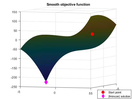
X0 = [2.5 -2.5];% Starting point.LB = [-5 -5];% Lower boundUB = [5 5];% Upper boundrange = [LB(1) UB(1); LB(2) UB(2)]; Objfcn = @smoothFcn;% Handle to the objective function.% Plot the smooth objective functionfig = figure('Color','w');showSmoothFcn(Objfcn,range); holdon;title('Smooth objective function');ph = [];ph值(1)= plot3(X0(1),X0(2),Objfcn(X0)+30,'or','MarkerSize',10,'MarkerFaceColor','r');holdoff;ax = gca; ax.CameraPosition = [-31.0391 -85.2792 -281.4265]; ax.CameraTarget = [0 0 -50]; ax.CameraViewAngle = 6.7937;% Add legend informationlegendLabels = {'Start point'}; lh = legend(ph,legendLabels,'Location','SouthEast');lp = lh.Position;lh。位置= [1-lp -0.005 (3)0.005 lp(3) lp(4)];

Runfminconon a Smooth Objective Function
The objective function is smooth (twice continuously differentiable). Solve the optimization problem using the Optimization Toolboxfminconsolver.fminconfinds a constrained minimum of a function of several variables. This function has a unique minimum at the pointx* = [-5,-5]where it has a valuef(x*) = -250.
Set options to return iterative display.
options = optimoptions(@fmincon,'Algorithm','interior-point','Display','iter');[Xop,Fop] = fmincon(Objfcn,X0,[],[],[],[],LB,UB,[],options) figure(fig); holdon;
First-order Norm of Iter F-count f(x) Feasibility optimality step 0 3 -1.062500e+01 0.000e+00 2.004e+01 1 6 -1.578420e+02 0.000e+00 5.478e+01 6.734e+00 2 9 -2.491310e+02 0.000e+00 6.672e+01 1.236e+00 3 12 -2.497554e+02 0.000e+00 2.397e-01 6.310e-03 4 15 -2.499986e+02 0.000e+00 5.065e-02 8.016e-03 5 18 -2.499996e+02 0.000e+00 9.708e-05 3.367e-05 6 21 -2.500000e+02 0.000e+00 1.513e-04 6.867e-06 7 24 -2.500000e+02 0.000e+00 1.161e-06 6.920e-08 Local minimum found that satisfies the constraints. Optimization completed because the objective function is non-decreasing in feasible directions, to within the value of the optimality tolerance, and constraints are satisfied to within the value of the constraint tolerance. Xop = -5.0000 -5.0000 Fop = -250.0000
Plot the final point
ph(2) = plot3(Xop(1),Xop(2),Fop,'dm','MarkerSize',10,'MarkerFaceColor','m');% Add a legend to plotlegendLabels = [legendLabels,'|fmincon| solution']; lh = legend(ph,legendLabels,'Location','SouthEast');lp = lh.Position;lh。位置= [1-lp -0.005 (3)0.005 lp(3) lp(4)]; holdoff;
Stochastic Objective Function
Now perturb the objective function by adding random noise.
rng(0,'twister')% Reset the global random number generatorpeaknoise = 4.5; Objfcn = @(x) smoothFcn(x,peaknoise);% Handle to the objective function.% Plot the objective function (non-smooth)fig = figure('Color','w');showSmoothFcn(Objfcn,range); title('Stochastic objective function') ax = gca; ax.CameraPosition = [-31.0391 -85.2792 -281.4265]; ax.CameraTarget = [0 0 -50]; ax.CameraViewAngle = 6.7937;

Runfminconon a Stochastic Objective Function
The perturbed objective function is stochastic and not smooth.fminconis a general constrained optimization solver which finds a local minimum using derivatives of the objective function. If you do not provide the first derivatives of the objective function,fminconuses finite differences to approximate the derivatives. In this example, the objective function is random, so finite difference estimates derivatives hence can be unreliable.fminconcan potentially stop at a point that is not a minimum. This may happen because the optimal conditions seems to be satisfied at the final point because of noise, orfminconcould not make further progress.
[Xop,Fop] = fmincon(Objfcn,X0,[],[],[],[],LB,UB,[],options) figure(fig); holdon;ph = [];ph值(1)= plot3(X0(1),X0(2),Objfcn(X0)+30,'or','MarkerSize',10,'MarkerFaceColor','r');ph(2) = plot3(Xop(1),Xop(2),Fop,'dm','MarkerSize',10,'MarkerFaceColor','m');% Add legend to plotlegendLabels = {'Start point','|fmincon| solution'}; lh = legend(ph,legendLabels,'Location','SouthEast');lp = lh.Position;lh。位置= [1-lp -0.005 (3)0.005 lp(3) lp(4)]; holdoff;
First-order Norm of Iter F-count f(x) Feasibility optimality step 0 3 -1.925772e+01 0.000e+00 2.126e+08 1 6 -7.107849e+01 0.000e+00 2.623e+08 8.873e+00 2 11 -8.055890e+01 0.000e+00 2.401e+08 6.715e-01 3 20 -8.325315e+01 0.000e+00 7.348e+07 3.047e-01 4 48 -8.366302e+01 0.000e+00 1.762e+08 1.593e-07 5 64 -8.591081e+01 0.000e+00 1.569e+08 3.111e-10 Local minimum possible. Constraints satisfied. fmincon stopped because the size of the current step is less than the value of the step size tolerance and constraints are satisfied to within the value of the constraint tolerance. Xop = -4.9628 2.6673 Fop = -85.9108

Runpatternsearch
Now minimize the stochastic objective function using the Global Optimization Toolboxpatternsearchsolver. Pattern search optimization techniques are a class of direct search methods for optimization. A pattern search algorithm does not use derivatives of the objective function to find an optimal point.
PSoptions = optimoptions(@patternsearch,'Display','iter');[Xps,Fps] = patternsearch(Objfcn,X0,[],[],[],[],LB,UB,PSoptions) figure(fig); holdon;ph(3) = plot3(Xps(1),Xps(2),Fps,'dc','MarkerSize',10,'MarkerFaceColor','c');% Add legend to plotlegendLabels = [legendLabels,'Pattern Search solution']; lh = legend(ph,legendLabels,'Location','SouthEast');lp = lh.Position;lh。位置= [1-lp -0.005 (3)0.005 lp(3) lp(4)]; holdoff
Iter Func-count f(x) MeshSize Method 0 1 -7.20766 1 1 3 -34.7227 2 Successful Poll 2 3 -34.7227 1 Refine Mesh 3 5 -34.7227 0.5 Refine Mesh 4 8 -96.0847 1 Successful Poll 5 10 -96.0847 0.5 Refine Mesh 6 13 -132.888 1 Successful Poll 7 15 -132.888 0.5 Refine Mesh 8 17 -132.888 0.25 Refine Mesh 9 20 -197.689 0.5 Successful Poll 10 22 -197.689 0.25 Refine Mesh 11 24 -197.689 0.125 Refine Mesh 12 27 -241.344 0.25 Successful Poll 13 30 -241.344 0.125 Refine Mesh 14 33 -241.344 0.0625 Refine Mesh 15 36 -241.344 0.03125 Refine Mesh 16 39 -241.344 0.01562 Refine Mesh 17 42 -242.761 0.03125 Successful Poll 18 45 -242.761 0.01562 Refine Mesh 19 48 -242.761 0.007812 Refine Mesh 20 51 -242.761 0.003906 Refine Mesh 21 55 -242.761 0.001953 Refine Mesh 22 59 -242.761 0.0009766 Refine Mesh 23 63 -242.761 0.0004883 Refine Mesh 24 67 -242.761 0.0002441 Refine Mesh 25 71 -242.761 0.0001221 Refine Mesh 26 75 -242.761 6.104e-05 Refine Mesh 27 79 -242.761 3.052e-05 Refine Mesh 28 83 -242.761 1.526e-05 Refine Mesh 29 87 -242.761 7.629e-06 Refine Mesh 30 91 -242.761 3.815e-06 Refine Mesh Iter Func-count f(x) MeshSize Method 31 95 -242.761 1.907e-06 Refine Mesh 32 99 -242.761 9.537e-07 Refine Mesh Optimization terminated: mesh size less than options.MeshTolerance. Xps = -4.9844 -4.5000 Fps = -242.7611
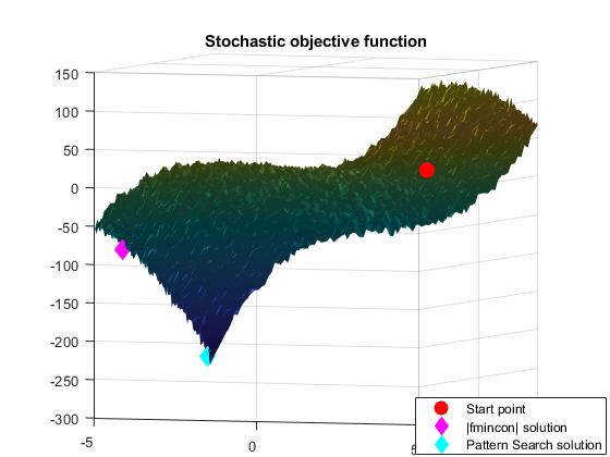
Pattern search is not as strongly affected by random noise in the objective function. Pattern search requires only function values and not the derivatives, hence noise (of some uniform kind) may not affect it. However, pattern search requires more function evaluation to find the true minimum than derivative based algorithms, a cost for not using the derivatives.
Related Topics
You can also select a web site from the following list:
Americas
- América Latina(Español)
- Canada(English)
- United States(English)
Europe
- Belgium(English)
- Denmark(English)
- Deutschland(Deutsch)
- España(Español)
- Finland(English)
- France(Français)
- Ireland(English)
- Italia(Italiano)
- Luxembourg(English)
- Netherlands(English)
- Norway(English)
- Österreich(Deutsch)
- Portugal(English)
- Sweden(English)
- Switzerland
- United Kingdom(English)