Modeling and Testing an LTE RF Receiver
This example demonstrates how to model and test an LTE RF receiver using LTE Toolbox™ and RF Blockset™.
Model Description
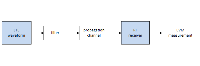
The figure below shows the main parts of this example. An LTE waveform is generated using the LTE Toolbox. This waveform is filtered and transmitted through a propagation channel before feeding it to the RF receiver model implemented with RF Blockset. This model is based on commercially available parts. EVM figures are then provided for the output of the RF receiver.
This example is implemented using MATLAB® and Simulink®, which interact at runtime. The functional partition is shown in the figure below
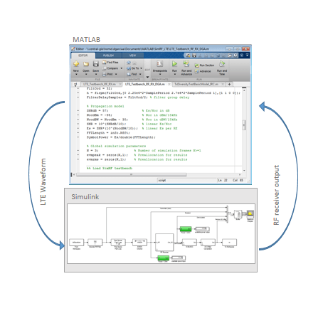
The MATLAB script implements the simulation test-bench, and the Simulink model is the device under test (DUT). LTE frames are streamed between the test-bench and the DUT.
Generate LTE Waveform
In this section we generate the LTE waveform using the LTE Toolbox. We use the reference measurement channel (RMC) R.6 as defined in TS 36.101 [1]. This RMC specifies a 25 resource elements (REs) bandwidth, equivalent to 5 MHz. A 64 QAM modulation is used. All REs are allocated. Additionally, OCNG noise is enabled in unused REs.
Only one frame is generated. This frame will then be repeated a number of times to perform the EVM measurements.
% Configuration TS 36.101 25 REs (5 MHz), 64-QAM, full allocationrmc = lteRMCDL('R.6'); rmc.OCNGPDSCHEnable ='On';% Create eNodeB transmission with fixed PDSCH datarng(2);% Fixed random seed (arbitrary)data = randi([0 1], sum(rmc.PDSCH.TrBlkSizes),1);% Generate 1 frame, to be repeated to simulate a total of N frames[tx, ~, info] = lteRMCDLTool(rmc, data);% 1 frame% Calculate the sampling period and the length of the frame.SamplePeriod = 1/info.SamplingRate; FrameLength = length(tx);
Initialize Simulation Components
This section initializes some of the simulation components:
Band limiting filter: design the filter coefficients, which will be used by the Simulink model. The filter has order 32, with passband frequency equal to 2.25 MHz, and stopband frequency equal to 2.7 MHz.
SNR and signal energy
Number of frames: this is the number of times the generated frame is repeated
Preallocate result vectors
% Band limiting interpolation filterFiltOrd = 32; h = firpm(FiltOrd,[0 2.25e6*2*SamplePeriod 2.7e6*2*SamplePeriod 1],[1 1 0 0]); FilterDelaySamples = FiltOrd/2;% filter group delay% Propagation modelSNRdB = 57;% Es/Noc in dBNocdBm = -98;% Noc in dBm/15kHzNocdBW = NocdBm - 30;% Noc in dBW/15kHz57SNR = 10^(SNRdB/10);% linear Es/NocEs = SNR*(10^(NocdBW/10));% linear Es per REFFTLength = info.Nfft; SymbolPower = Es/double(FFTLength);% Number of simulation frames N>=1N = 3;% Preallocate vectors for results for N-1 frames% EVM is not measured in the first frame to avoid transient effectsevmpeak = zeros(N-1,1);% Preallocation for resultsevmrms = zeros(N-1,1);% Preallocation for results
Load RF Blockset Testbench
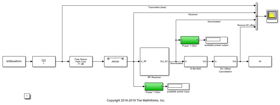
This section loads the Simulink model shown below. This model includes the following components:
Reading the LTE waveform and the sampling period from the workspace
Bandlimiting filtering
Channel model: this includes free space path loss and AWGN
RF receiver, including direct conversion demodulator
ADC and DC offset cancellation
Save results to workspace
% Specify and open Simulink modelmodel ='RFLTEReceiverModel'; disp('Starting Simulink'); open_system(model);
Starting Simulink
RF Receiver Model
The RF receiver model includes the elements shown below
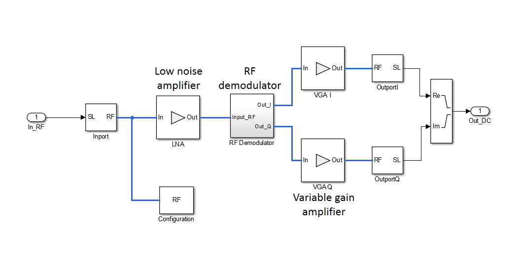
The RF demodulator includes the following components and is shown below:
Local oscillator (LO) and phase noise model
Phase shift for I and Q components generator
Mixers

Simulate Frames
This section simulates the specified number of frames. This is done in two stages:
Simulate the first frame
Simulate the rest of the frames in a loop
The reason for splitting the processing in these two stages is to simplify the code. During the processing of the first frame we need to take into account the delay of the band limiting filter. This is not the case for subsequent frames, since the filter state is maintained between frames. Therefore, the length of the first frame has to be increased slightly to take into account the delay introduced by the filter.
模拟第一LTE框架
As mentioned for the first simulated frame we need to increase the length of the signal fed to the Simulink model to compensate for the delay introduced by the filter. Next we launch the simulation of the Simulink model without loading any initial state. After processing the first frame with the Simulink model, its state (xFinal) is stored and assigned toxInitialfor the next time the model is run.
The output of the Simulink model is stored in the variablerx, which is available in the workspace. Any delays introduced to this signal are removed after performing synchronization. The EVM is measured on the resulting waveform.
% Generate test data for RF receivertime = (0:FrameLength+FilterDelaySamples)*SamplePeriod;% Append to the end of the frame enough samples to compensate for the delay% of the filtertxWaveform = timeseries([tx; tx(1:FilterDelaySamples+1)],time);% Simulate RF Blockset model of RF RXset_param(model,'LoadInitialState','off'); disp('Simulating LTE frame 1 ...'); sim(model, time(end));% Save the final state of the model in xInitial for next frame processingxInitial = xFinal;% Synchronize to received waveformOffset = lteDLFrameOffset(rmc,squeeze(rx),'TestEVM');% In this case Offset = FilterDelaySamples therefore the following% frames do not require synchronization
Simulating LTE frame 1 ...
Simulate Successive LTE Frames
现在其余的帧可以模拟。第一个, the model state is set using the value stored inxInitialat the output of the previous iteration.
% Load state after execution of previous frame. Since we are repeating the% same frame the model state will be the same after every frame execution.set_param(model,'LoadInitialState','on','InitialState','xInitial');% Modify input vector to take into account the delay of the bandlimiting% filterRepeatFrame = [tx(FilterDelaySamples+1:end); tx(1:FilterDelaySamples+1)]; EVMalg.EnablePlotting ='Off'; cec.PilotAverage ='TestEVM';forn = 2:N% for all remaining frames% Generate datatime = ( (n-1)*FrameLength+(0:FrameLength) + FilterDelaySamples)*SamplePeriod; txWaveform = timeseries(RepeatFrame,time);% Execute Simulink RF Blockset testbenchdisp(['Simulating LTE frame ',num2str(n),' ...']); sim(model, time(end)); xInitial = xFinal;% Save model state% Compute and display EVM measurementsevmmeas = hPDSCHEVM(rmc,cec,squeeze(rx),EVMalg); evmpeak(n-1) = evmmeas.Peak; evmrms(n-1) = evmmeas.RMS;end
Simulating LTE frame 2 ... Low edge EVM, subframe 0: 2.908% High edge EVM, subframe 0: 2.919% Low edge EVM, subframe 1: 2.653% High edge EVM, subframe 1: 2.667% Low edge EVM, subframe 2: 2.927% High edge EVM, subframe 2: 2.935% Low edge EVM, subframe 3: 3.429% High edge EVM, subframe 3: 3.423% Low edge EVM, subframe 4: 2.935% High edge EVM, subframe 4: 2.950% Low edge EVM, subframe 6: 3.100% High edge EVM, subframe 6: 3.096% Low edge EVM, subframe 7: 3.143% High edge EVM, subframe 7: 3.145% Low edge EVM, subframe 8: 3.188% High edge EVM, subframe 8: 3.189% Low edge EVM, subframe 9: 3.151% High edge EVM, subframe 9: 3.148% Averaged low edge EVM, frame 0: 3.057% Averaged high edge EVM, frame 0: 3.061% Averaged EVM frame 0: 3.061% Averaged overall EVM: 3.061% Simulating LTE frame 3 ... Low edge EVM, subframe 0: 2.918% High edge EVM, subframe 0: 2.922% Low edge EVM, subframe 1: 2.732% High edge EVM, subframe 1: 2.738% Low edge EVM, subframe 2: 3.044% High edge EVM, subframe 2: 3.044% Low edge EVM, subframe 3: 3.475% High edge EVM, subframe 3: 3.444% Low edge EVM, subframe 4: 2.914% High edge EVM, subframe 4: 2.923% Low edge EVM, subframe 6: 3.139% High edge EVM, subframe 6: 3.137% Low edge EVM, subframe 7: 3.186% High edge EVM, subframe 7: 3.187% Low edge EVM, subframe 8: 3.116% High edge EVM, subframe 8: 3.110% Low edge EVM, subframe 9: 3.089% High edge EVM, subframe 9: 3.083% Averaged low edge EVM, frame 0: 3.077% Averaged high edge EVM, frame 0: 3.073% Averaged EVM frame 0: 3.077% Averaged overall EVM: 3.077%
According to TS 36.104 [2], the maximum EVM when the constellation is 64-QAM is 8%. As the overall EVM, around 3%, is lower than 8%, this measurement falls within the requirements of TS 36.104 [2].
Visualize Measured EVM
This section plots the measured peak and RMS EVM for each simulated frame.
figure; plot((2:N), 100*evmpeak,'o-') title('EVM peak %'); xlabel('Number of frames'); figure; plot((2:N), 100*evmrms,'o-'); title('EVM RMS %'); xlabel('Number of frames');


Cleaning Up
Close the Simulink model and remove the generated files.
bdclose(model); clear([model,'_acc']);
Appendix
This example uses the following helper functions:
Selected Bibliography
3GPP TS 36.101 "User Equipment (UE) radio transmission and reception"
3GPP TS 36.104 "E-UTRA; Base Station (BS) radio transmission and reception"3rd Generation Partnership Project; Technical Specification Group Radio Access Network.
Select a Web Site
Choose a web site to get translated content where available and see local events and offers. Based on your location, we recommend that you select:.
Selectweb site你也可以从下面选择一个网站list:
Americas
- América Latina(Español)
- Canada(English)
- United States(English)
Europe
- Belgium(English)
- Denmark(English)
- Deutschland(Deutsch)
- España(Español)
- Finland(English)
- France(Français)
- Ireland(English)
- Italia(Italiano)
- Luxembourg(English)
- Netherlands(English)
- Norway(English)
- Österreich(Deutsch)
- Portugal(English)
- Sweden(English)
- Switzerland
- United Kingdom(English)