非均匀热流多域几何中的热传导
这个例子演示了如何对由三层不同材料制成的空心球进行三维瞬态热传导分析。
球体受到不均匀的外部热流的影响。
这个问题的物理性质和几何描述在Singh, Jain,和Rizwan-uddin(见参考文献),也有一个解析解这个问题。球体的内表面的温度在任何时候都是零。外半球为正 值具有非均匀热流,定义为
和 为球面上各点的方位角和仰角。一开始,球面上所有点的温度都是零。
建立瞬态热分析的热模型。
thermalmodel = createpde (“热”,瞬态的);
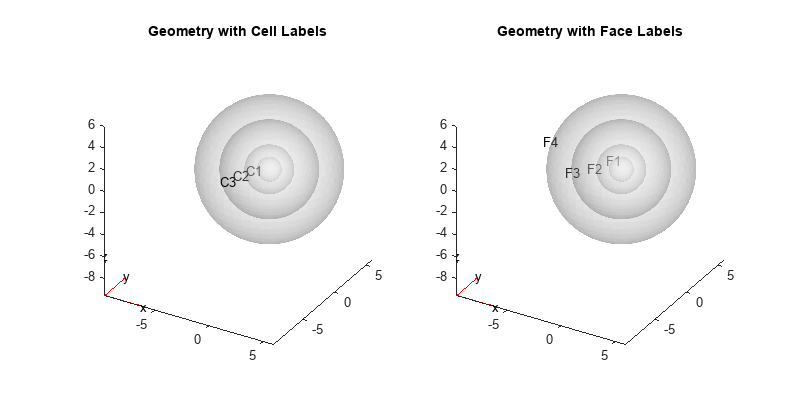
创建一个多层球体使用multisphere函数。将结果几何图形赋给热模型。这个球体有三层材料,内芯是空心的。
通用= multisphere(1、2、4、6,“空白”,真的,假的,假的,假的);thermalmodel。几何=通用;
绘制几何图形并显示单元格标签和面标签。使用一个FaceAlpha0.25,这样内层的标签是可见的。
图(“位置”[10800400]);次要情节(1、2、1)pdegplot (thermalmodel,“FaceAlpha”, 0.25,“CellLabel”,“上”)标题(“带有单元格标签的几何图形”次要情节(1、2、2)pdegplot (thermalmodel,“FaceAlpha”, 0.25,“FaceLabel”,“上”)标题(“带有面部标签的几何图形”)
为几何体生成一个网格。选择一个足够粗的网格尺寸来加速求解,但又足够细的网格尺寸来合理准确地表示几何图形。
generateMesh (thermalmodel“Hmax”1);
为球体的每一层指定导热系数、质量密度和比热。材料属性是无量纲值,不是由真实的材料属性给出的。
thermalProperties (thermalmodel“细胞”,1,“ThermalConductivity”,1,...“MassDensity”,1,...“SpecificHeat”1);thermalProperties (thermalmodel“细胞”,2,“ThermalConductivity”,2,...“MassDensity”,1,...“SpecificHeat”, 0.5);thermalProperties (thermalmodel“细胞”3,“ThermalConductivity”,4,...“MassDensity”,1,...“SpecificHeat”, 4/9);
指定边界条件。最内面的温度一直是零。
thermalBC (thermalmodel“脸”,1,“温度”, 0);
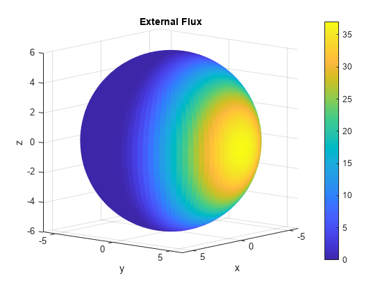
球体的外表面有一个外部热流。用热边界条件的函数形式来定义热流。
函数Qflux = externalHeatFlux(region,~)
[θ,φ~]= cart2sph (region.x, region.y region.z);
= /2 -;%变换为0 <= theta <= PI
id = phi > 0;
Qflux = 0(大小(region.x));
Qflux (ids) =θ(ids) ^ 2。*(π-θ(ids)) ^ 2 ^ 2 *φ(ids)。*(π-φ(ids)) ^ 2;
结束
在表面画出通量。
(φ,θ,r) = meshgrid (linspace(0, 2 *π),linspace(-π/ 2π/ 2),6);[x, y, z] = sph2cart(φ,θ,r);地区。x = x;地区。y = y;地区。z = z;通量= externalHeatFlux(地区、[]);图冲浪(x, y, z,通量,“线型”,“没有”)轴平等的视图(130年,10)colorbar包含“x”ylabel“y”zlabel“z”标题(“外部流量”)
将这个边界条件包含到模型中。
thermalBC (thermalmodel“脸”,4,...“HeatFlux”@externalHeatFlux,...矢量化的,“上”);
定义初始温度在所有点都为零。
thermalIC (thermalmodel 0);
定义时间步向量,求解瞬态热问题。
tlist =[0、2、5:5:50];R =解决(thermalmodel tlist);
若要多次绘制等高线,且等高线在所有图中都是相同的,则需要确定溶液中的温度范围。最低温度是零,因为它是球体内表面的边界条件。
Tmin = 0;
从最后的时间步解中找到最高温度。
达峰时间= max (R.Temperature(:,结束));
绘制范围内的等高线Tmin来达峰时间在泰晤士报tlist.
h =图;为i = 1:numel(tlist)“ColorMapData”,R.Temperature(:,i)) caxis([Tmin,Tmax]) view(130,10) title([“时间温度”num2str (tlist (i))));M (i) = getframe;结束

要在计算机上运行此示例时查看轮廓的影片,请执行以下行:
电影(M, 2)
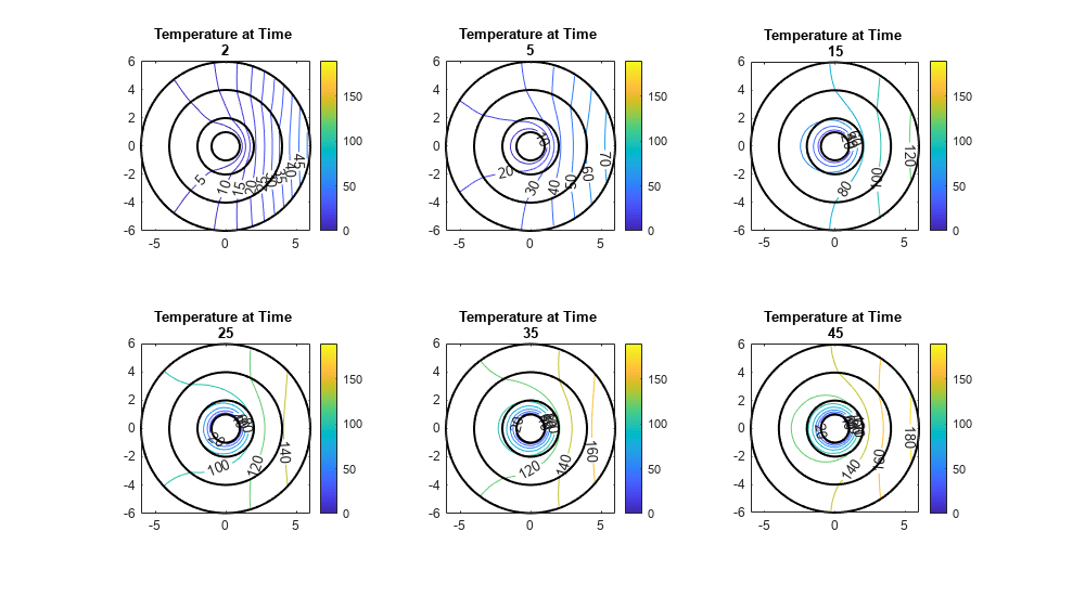
观察横截面上的温度曲线。首先,定义一个矩形网格上的点 飞机在哪里 .
[YG, ZG] = meshgrid (linspace (6100), linspace (6100);XG = 0(大小(YG));
插值网格点的温度。对几个时间步长进行插值,观察温度轮廓的变化。
tIndex =[2、3、5、7、9、11);varNames = {“Time_index”,“Time_step”};index_step =表(tIndex。”,tlist (tIndex)。’,“VariableNames”, varNames);disp (index_step);
Time_index Time_step __________ _________ 2 2 3 5 5 15 7 25 9 35 11 45
TG = interpolateTemperature (R, XG, YG、ZG tIndex);
在横截面上定义几何球形层。
t = linspace(0, 2 *π);ylayer1 = cos (t);zlayer1 =罪(t);ylayer2 = 2 * cos (t);zlayer2 = 2 * sin (t);ylayer3 = 4 * cos (t);zlayer3 = 4 * sin (t);ylayer4 = 6 * cos (t);zlayer4 = 6 * sin (t);
绘制范围内的等高线Tmin来达峰时间对应于时间指标的时间步长tIndex.
图(“位置”, 10、10、1000、550);为i = 1:numel(tIndex) subplot(2,3,i) contour(YG,ZG,重塑(TG(:,i),size(YG)),“ShowText”,“上”) colorbar标题(“时间温度”num2str (tlist (tIndex (i)))));持有在caxis ([Tmin,达峰时间])轴平等的%绘制球面层边界供参考。情节(ylayer1 zlayer1,“k”,“线宽”1.5)情节(ylayer2 zlayer2,“k”,“线宽”1.5)情节(ylayer3 zlayer3,“k”,“线宽”1.5)情节(ylayer4 zlayer4,“k”,“线宽”, 1.5)结束
参考
辛格、苏尼特、p·k·杰恩和里兹万·乌丁。多层球体中三维非稳态热传导的解析解。ASME。[j] .清华大学学报(自然科学版),2016,43(4):457 - 461。
你也可以从以下列表中选择一个网站: