Custom Transformer (B-H Curve)
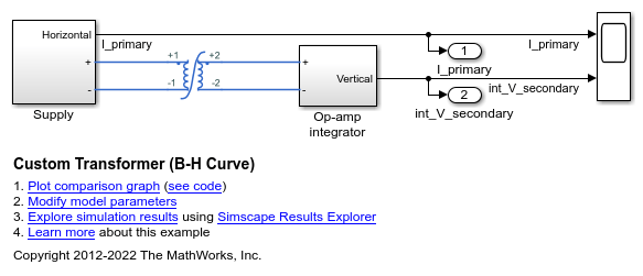
This example shows calculation and confirmation of a nonlinear transformer core magnetization characteristic. Starting with fundamental parameter values, the core characteristic is derived. This is then used in a Simscape™ model of an example test circuit which can be used to plot the core magnetization characteristic on an oscilloscope. Model outputs are then compared to the known values.
Open Model
modelName ='ee_custom_transformer'; open_system( modelName );

Specification of Parameters
Fundamental parameter values used as the basis for subsequent calculations:
Permeability of free space,

Relative permeability of core,

Number of primary turns,

Number of secondary turns,

Effective magnetic core length,

Effective magnetic core cross-sectional area,

Core saturation begins,

Core fully saturated,

mu_0 = pi*4e-7; mu_r = 3000; N1 = 100; N2 = 200; le = 0.1; Ae = 1e-4; B_sat_begin = 0.6; B_sat = 1.2;
Calculate Magnetic Flux Density Versus Magnetic Field Strength Characteristic
地点:
Magnetic flux density,

Magnetic field strength,

Linear representation:
Nonlinear representation (including coefficient, a):
%使用linear representation to find value of H corresponding to B_sat_beginH_sat_begin = B_sat_begin/(mu_0*mu_r);% Rearrange nonlinear representation to calculate coefficient, aa = atanh( B_sat_begin/B_sat )/H_sat_begin;% Nonlinear representationH_nonlinear = -750:25:750; B_nonlinear = B_sat*tanh(a*H_nonlinear);
Use Parameters in Simscape Model
现在可以使用的参数计算的Sim卡scape model. Once simulated, the model is set to output a Simscape logging variable, simlog_ee_custom_transformer, and some signals using output ports, yout. Circuit parameters are:
Voltage source magnitude,

Voltage source frequency,

Voltage source resistance,

Operational amplifier input resistance,

Operational amplifier feedback resistance,

Operational amplifier feedback capacitance,

% Circuit parametersVs = 10; Freq_Hz = 60; R_Vs = 10; R_1 = 1e3; R_2 = 1e6; C_2 = 1e-6;% Simulate modelsimOut = sim( modelName ); yout = get(simOut,'yout'); simlog = get(simOut,'simlog_ee_custom_transformer');% Collect internal Simscape logging data for comparisonI_simscape = simlog.Transformer_B_H_curve.L_m.i.series.values; phi_simscape = simlog.Transformer_B_H_curve.L_m.phi.series.values;% Collect model output data for comparison (as used for oscilloscope)I_primary = yout(:,1); int_V_secondary = yout(:,2);
Calculations on Logging and Output Data
The data needs to be processed to provide the Magnetic field strength and Magnetic flux density data for comparison. Where:
Magnetomotive force,

Magnetic flux,

Operational amplifier input voltage,

Operational amplifier output voltage,

Equations to be used are as follows:
% Internal logging dataH_simscape = I_simscape.*N1./le; B_simscape = phi_simscape./Ae;% Oscilloscope scaling and model output dataH_measured = I_primary.*N1./le; phi_measured = (int_V_secondary.*R_1.*C_2)./N2; B_measured = phi_measured./Ae;
Conclusion
The three characteristics can now be overlaid:
Defined characteristic: calculated from fundamental parameters
Characteristic from logging: calculated from internal Simscape logging data
Characteristic from measurement: obtained by measurement and calculation using electronic test circuit
Due to leakage and parasitic parameters, the characteristic obtained from the electronic test circuit differs to the defined characteristic. However, the test circuit and its parameterization is shown to find the characteristic for the given transformer within suitable tolerances.
if~exist('h1_ee_custom_transformer','var') ||...~isgraphics(h1_ee_custom_transformer,'figure') h1_ee_custom_transformer = figure('Name','ee_custom_transformer');endfigure(h1_ee_custom_transformer) clf(h1_ee_custom_transformer) plot(...H_nonlinear,...B_nonlinear,...'o',...H_simscape,...B_simscape,...H_measured,...B_measured,...“- - -”,...'LineWidth',2); grid('on'); title('Transformer B-H Curve'); xlabel('Magnetic Field Strength, H (A/m)'); ylabel('Magnetic Flux Density, B (T)'); legend('Calculated','Simulated',...'From Sensor','Location','NorthWest');

Results from Real-Time Simulation
This example has been tested on a Speedgoat Performance real–time target machine with an Intel® 3.5 GHz i7 multi–core CPU. This model can run in real time with a step size of 50 microseconds.


