开始

TypefilterDesignerat the MATLAB command prompt:

> > filterDesigner

ATip of the Daydialog displays with suggestions for using Filter Designer. Then, the GUI displays with a default filter.

The GUI has three main regions:

The upper half of the GUI displays information on filter specifications and responses for the current filter. The Current Filter Information region, in the upper left, displays filter properties, namely the filter structure, order, number of sections used and whether the filter is stable or not. It also provides access to the Filter manager for working with multiple filters.

The Filter Display region, in the upper right, displays various filter responses, such as, magnitude response, group delay and filter coefficients.

The lower half of the GUI is the interactive portion of Filter Designer. The Design Panel, in the lower half is where you define your filter specifications. It controls what is displayed in the other two upper regions. Other panels can be displayed in the lower half by using the sidebar buttons.

The tool includes Context-sensitive help. You can right-click or click theWhat's This?button to get information on the different parts of the tool.

Designing a Filter

We will design a low pass filter that passes all frequencies less than or equal to 20% of the Nyquist frequency (half the sampling frequency) and attenuates frequencies greater than or equal to 50% of the Nyquist frequency. We will use an FIR Equiripple filter with these specifications:

To implement this design, we will use the following specifications:

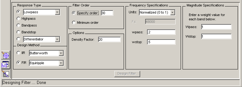
1. SelectLowpassfrom the dropdown menu underResponse TypeandEquirippleunderFIR Design Method. In general, when you change the Response Type or Design Method, the filter parameters and Filter Display region update automatically.

2. SelectSpecify orderin theFilter Orderarea and enter30.

3. The FIR Equiripple filter has aDensity Factoroption which controls the density of the frequency grid. Increasing the value creates a filter which more closely approximates an ideal equiripple filter, but more time is required as the computation increases. Leave this value at 20.

4. SelectNormalized (0 to 1)in the Units pull down menu in theFrequency Specificationsarea.

5. Enter0.2forwpassand0.5forwstopin theFrequency Specificationsarea.

6.WpassandWstop, in theMagnitude Specificationsarea are positive weights, one per band, used during optimization in the FIR Equiripple filter. Leave these values at 1.

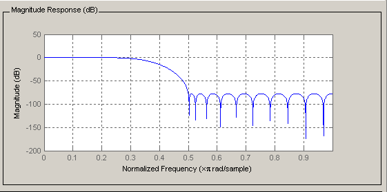
7. After setting the design specifications, click theDesign Filterbutton at the bottom of the GUI to design the filter.

The magnitude response of the filter is displayed in the Filter Analysis area after the coefficients are computed.

Viewing other Analyses

Once you have designed the filter, you can view the following filter analyses in the display window by clicking any of the buttons on the toolbar:

In order from left to right, the buttons are

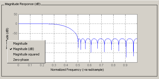
Changing Axes Units

You can change the x- or y-axis units by right-clicking the mouse on an axis label and selecting the desired units. The current units have a check mark.

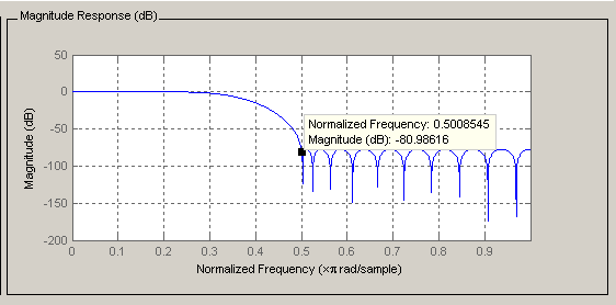
Marking Data Points

In the Display region, you can click on any point in the plot to add a data marker, which displays the values at that point. Right-clicking on the data marker displays a menu where you can move, delete or adjust the appearance of the data markers.

Optimizing the Design

To minimize the cost of implementation of the filter, we will try to reduce the number of coefficients by usingMinimum Orderoption in the design panel.

Change the selection inFilter OrdertoMinimum Orderin the Design Region and leave the other parameters as they are.

Click theDesign Filter按钮设计the new filter.

As you can see in the Current Filter Information area, the filter order decreased from 30 to 16, the number of ripples decreased and the transition width became wider. The passband and the stopband specifications still meet the design criteria.

Changing Analyses Parameters

By right-clicking on the plot and selecting Analysis Parameters, you can display a dialog box for changing analysis-specific parameters. (You can also select Analysis Parameters from the Analysis menu.)

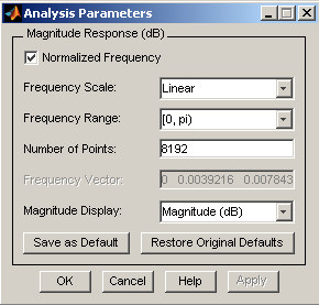
To save the displayed parameters as the default values, clickSave as Default. To restore the MATLAB-defined default values, clickRestore Original Defaults.

Exporting the Filter

Once you are satisfied with your design, you can export your filter to the following destinations:

SelectExportfrom theFilemenu.

When you choose to export to the MATLAB workspace or to a MAT-file, you can export the filter as coefficients. If a DSP System Toolbox™ is available you can also export your filter as a System object.

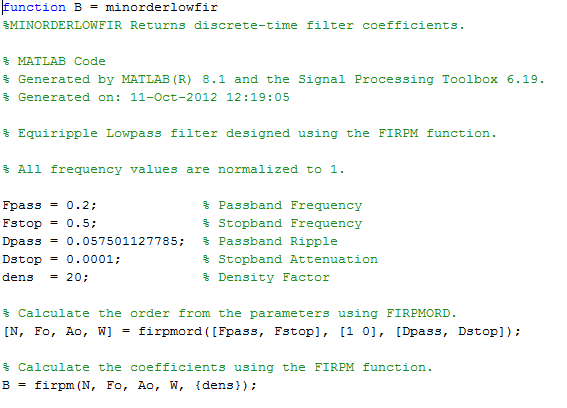
Generating a MATLAB File

Filter Designer allows you to generate MATLAB code to re-create your filter. This enables you to embed your design into existing code or automate the creation of your filters in a script.

SelectGenerate MATLAB codefrom theFilemenu, chooseFilter Design Function并指定生成的文件名MATLAB code dialog box.

The following code was generated from the minimum order filter we designed above:

Quantizing a Filter

If you have the DSP System Toolbox™ installed, theSet quantization parameterspanel is available on the sidebar:

You can use this panel to quantize and analyze double-precision filters. With the DSP System Toolbox you can quantize from double-precision to single-precision. If you have the Fixed-Point Designer, you can quantize filters to fixed-point precision. Note that you cannot mix floating-point and fixed-point arithmetic in your filter.

Targets

TheTargetsmenu of Filter Designer allows you to generate various types of code representing your filter. For example, you can generate C header files, XILINX coefficients(COE) files (with the DSP System Toolbox) and VHDL, Verilog along with test benches (with Filter Design HDL Coder™).

Additional Features

Filter Designer also integrates additional functionality from these other MathWorks™ products: