通过Feynman-Kac公式模拟随机过程

Open Live Script

this example obtains the partial differential equation that describes the expected final price of an asset whose price is a stochastic process given by a stochastic differential equation.

涉及的步骤是：

Define Parameters of the Model Using Stochastic Differential Equations
应用ITO的规则
Solve Feynman-Kac Equation
计算预期出售资产的时间

1。Define Parameters of the Model Using Stochastic Differential Equations

资产价格的模型x（t）deFined in the time interval[0,T]is a stochastic process defined by a stochastic differential equation of the form $d X = μ （（ t ，，，， X ） d t + σ （（ t ，，，， X ） d b （（ t ）$ ，，，，whereb（t）is the Wiener process with unit variance parameter.

Create the symbolic variablet一个nd the following symbolic functions:

r（（t）is a continuous function representing a spot interest rate. This rate determines the discount factor for the final payoff at the timet。
你（（t，，，，X）是计算为折扣未来价格的预期价值 $X （（ t ） eXp （（ - \int_{t}^{t} r （（ t ） d t ）$ 你nder the conditionx（t）=X。
$μ （（ t ，，，， X ）$ 一个nd $σ （（ t ，，，， X ）$ 是随机过程的漂移和扩散x（t）。

symsMu（t，x）西格玛（（t，，，，X）r（t，x）u（t，x）t

根据Feynman-Kac定理的说法你满足the partial differential equation $\frac{\partial 你}{\partial t} + \frac{σ^{2}}{2} \frac{\partial^{2} 你}{\partial X^{2}} + μ \frac{\partial 你}{\partial X} - 你 r = 0$ with a final condition at timet。

eq = diff(u, t) + sigma^2*diff(u, X, X)/2 + mu*diff(u, X) - u*r;

the numerical solverpdepe适合初始条件。要将最终条件转换为初始条件，请通过设置应用时间逆转v（（t，，，，X）=你（（t-t, X)。

symsv（（t，，，，X）eq2 = subs（eq，{u，t}，{v（t -t -t，x），t -t}）;eq2 = feval（Symengine，'改写'，，，，eq2，，，，'diff'）

eq2=
                  
                    $\frac{{σ （（ t - t ，，，， X ）}^{2} \frac{\partial^{2}}{\partial X^{2}} v （（ t ，，，， X ）}{2} + μ （（ t - t ，，，， X ） \frac{\partial}{\partial X} v （（ t ，，，， X ） - \frac{\partial}{\partial t} v （（ t ，，，， X ） - v （（ t ，，，， X ） r （（ t - t ，，，， X ）$

the solverpdepe需要以下形式的部分微分方程。这里的系数C，，，，F，，，，一个nds一个reF你nctions ofX，，，，t，，，，v，，，，一个nd $\partial v / \partial X$ 。

$C \frac{\partial v}{\partial t} = \frac{\partial F}{\partial X} + s$

to be able to solve the equationeq2with thepdepesolver, mapeq2为此形式。首先，提取系数和术语eq2。

symsdvtdvXXeq3 = subs(eq2, {diff(v, t), diff(v, X, X)}, {dvt, dvXX}); [k,terms] = coeffs(eq3, [dvt, dvXX])

k=
                  
                    $（（ \begin{array}{c} - 1 & \frac{{σ （（ t - t ，，，， X ）}^{2}}{2} & μ （（ t - t ，，，， X ） \frac{\partial}{\partial X} v （（ t ，，，， X ） - v （（ t ，，，， X ） r （（ t - t ，，，， X ） \end{array} ）$

条款=
                   $（（ \begin{array}{c} dvt & dvXX & 1 \end{array} ）$

现在，您可以重写eq2作为k（（1）*terms(1) + k(2)*terms(2) + k(3)*terms(3) = 0。Moving the term with the time derivative to the left side of the equation, you get

$\frac{\partial v}{\partial t} = k （（ 2 ） \frac{\partial^{2} v}{\partial X^{2}} + k （（ 3 ）$

Manually integrate the right side by parts. The result is

$\frac{\partial}{\partial X} （（ k （（ 2 ） \frac{\partial v}{\partial X} ） + k （（ 3 ） - \frac{\partial v}{\partial X} \frac{\partial k （（ 2 ）}{\partial X}$

therefore, to writeeq2以适合pdepe，，，，你sethe following parameters:

C=1;F=k（（2）* diff(v, X); s = k(3) - diff(v, X) * diff(k(2), X);

2。应用ITO的规则

资产价格遵循乘法过程。也就是说，价格的对数可以用SDE来描述，但是价格本身的预期值是值得的，因为它描述了利润，因此我们需要后者的SDE。

通常，如果是随机过程Xis given in terms of an SDE, then Ito's rule says that the transformed processG（（t，，，，X）满足

$d G = （（ μ \frac{d G}{d X} + \frac{σ^{2}}{2} \frac{d^{2} G}{d X^{2}} + \frac{d G}{d t} ） d t + \frac{d G}{d X} σ d b （（ t ）$

我们假设价格的对数是由一维添加剂布朗尼运动给出的，也就是说mu一个nd西格玛是常数。定义应用ITO规则的函数，并使用它将加性布朗运动转变为几何布朗尼运动。

ito = @（MU，Sigma，G，T，X）。。。deal（mu * diff（g，x） + sigma^2/2 * diff（g，x，x） + diff（g，t），。。。diff(G, X) * sigma ); symsmu0Sigma0[mu1, sigma1] = ito(mu0, sigma0, exp(X), t, X)

mu1 =
                  
                    $\frac{e^{X} {σ_{0}}^{2}}{2} + μ_{0} e^{X}$

sigma1 =
                   $σ_{0} e^{X}$

ReplaceeXp(X)经过y。

symsymu1 = subs(mu1, X, log(Y)); sigma1 = subs(sigma1, X, log(Y)); f = f(t, log(Y)); s = s(t, log(Y));

为简单起见，假设利率为零。这是一个特殊情况，也称为kolmogorov向后方程。

r0=0;C=s你bs（（C，，，， {mu, sigma}, {mu1, sigma1}); s = subs(s, {mu, sigma, r}, {mu1, sigma1, r0}); f = subs(f, {mu, sigma}, {mu1, sigma1});

3。Solve Feynman-Kac Equation

beFore you can convert symbolic expressions to MATLAB function handles, you must replace function calls, such asdiff(v(t, X), X)一个ndv（（t，，，，X），带变量。您可以使用任何有效的MATLAB变量名称。

symsDVDXv;dvx = diff（v，x）;c = subs（c，{dvx，v}，{dvdx，v}）;f = subs（f，{dvx，v}，{dvdx，v}）;s = subs（s，{dvx，v}，{dvdx，v}）;

对于平坦的几何形状（翻译对称），设置以下值：

m = 0;

Also, assign numeric values to symbolic parameters.

muvalue = 0; sigmavalue = 1; c0 = subs(c, {mu0, sigma0}, {muvalue, sigmavalue}); f0 = subs(f, {mu0, sigma0}, {muvalue, sigmavalue}); s0 = subs(s, {mu0, sigma0}, {muvalue, sigmavalue});

利用matlabFunctionto create a function handle. Pass the coefficientsC0，，，，F0，，，，一个nds0in the form required bypdepe，，，，namely, a function handle with three output arguments.

feynmankacpde = matlabFunction（C0，F0，S0，'vars'，，，，[t, Y, V, dvdx])

FeynmanKacPde =F你nction_handle with value:@(t,Y,V,dvdx)deal(1.0,0.0,0.0)

As the final condition, take the identity mapping. That is, the payoff at time $t$ is given by the asset price itself. You can modify this line in order to investigate derivative instruments.

FeynmanKacIC = @(x) x;

PDE的数值求解只能应用于有限域。因此，您必须指定边界条件。假设该资产在其价格上涨或跌至一定限制的那一刻出售，因此解决方案v必须满足X -V = 0在边界点X。you can choose another boundary condition, for example, you can useV = 0to model knockout options. The zeroes in the second and fourth output indicate that the boundary condition does not depend on $\frac{d v}{d X}$ 。

FeynmanKacBC = @(xl, vl, xr, vr, t)。。。de一个l(xl - vl, 0, xr - vr, 0);

Choose the space grid, which is the range of values of the priceX。Set the left boundary to zero: it is not reachable by a geometric random walk. Set the right boundary to one: when the asset price reaches this limit, the asset is sold.

Xgrid = linspace(0, 1, 101);

选择时间网格。由于一开始就应用时间逆转，它表示剩下的时间直到最后一次t。

tgrid = linspace（0，1，21）;

解决方程。

sol = pdepe(m,FeynmanKacPde,FeynmanKacIC,FeynmanKacBC,xgrid,tgrid);

绘制解决方案。预期的销售价格几乎线性地取决于时间的价格t，，，，一个nd also weakly ont。

冲浪（XGRID，TGRID，SOL）标题（“预期的资产销售价格”）；Xlabel（'price'）；ylabel('time'）；Zlabel（'expected final price'）；

图包含一个轴对象。轴对象具有标题的预期销售价格，其中包含类型表面的对象。

the state of a geometric Brownian motion with drift $μ 1$ 一个ttimet是一个对数正态分布的随机变量eXpected value $eXp （（ μ_{1} t ）$ 乘以其初始值。这描述了由于达到限制而从未出售的资产的预期售价。

Expected = transpose(exp(tgrid./2)) * xgrid;

Dividing the solution obtained above by that expected value shows how much profit is lost by selling prematurely at the limit.

sol2 = sol./Expected; surf(xgrid, tgrid, sol2) title('Ratio of expected final prices: with / without sales order at x=1'）Xlabel（'price'）；ylabel('time'）；Zlabel（'ratio of final prices'）；

图包含一个轴对象。轴对象具有预期最终价格的标题比：x = 1的销售订单有 /不带有类型表面对象。

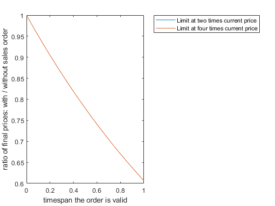
例如,预期收益的比例of an asset for which a limit sales order has been placed and the same asset without sales order over a timespant，，，，作为一个F你nction oft。考虑分别是当前价格的两倍和四倍的订单限额的情况。

plot(tgrid, sol2(:, xgrid == 1/2)); holdon绘图（tgrid，sol2（：，xgrid == 1/4））;传奇（“限制当前价格两倍”，，，，“限制为当前价格的四倍”）；Xlabel（'timespan the order is valid'）；ylabel('ratio of final prices: with / without sales order'）；抓住离开

图包含一个轴对象。the axes object contains 2 objects of type line. These objects represent Limit at two times current price, Limit at four times current price.

4。计算预期出售资产的时间

这是一本教科书结果，即达到限制并出售资产的预期退出时间由以下等式给出：

symsy（（X）eXitTimeEquation(X) = subs(eq, {r, u}, {0, y(X)}) == -1

eXitTimeEquation(X) =
                  
                    $\frac{{σ （（ t ，，，， X ）}^{2} \frac{\partial^{2}}{\partial X^{2}} y （（ X ）}{2} + μ （（ t ，，，， X ） \frac{\partial}{\partial X} y （（ X ） = - 1$

此外，y边界必须为零。为了mu一个nd西格玛，插入正在考虑的实际随机过程：

eXitTimeGBM = subs(subs(exitTimeEquation, {mu, sigma}, {mu1, sigma1}), Y, X)

eXitTimeGBM(X) =
                  
                    $(\frac{X {σ_{0}}^{2}}{2} + X μ_{0}) \frac{\partial}{\partial X} y （（ X ） + \frac{X^{2} {σ_{0}}^{2} \frac{\partial^{2}}{\partial X^{2}} y （（ X ）}{2} = - 1$

Solve this problem for arbitrary interval borders一个一个ndb。

syms一个battitime = dsolve（eTittimeGBM，y（a）== 0，y（b）== 0）

出口=
                  
                    $\begin{array}{l} \frac{2 μ_{0} σ_{5} \log （（ b ） - 2 μ_{0} σ_{4} \log （（ 一个 ） + {一个}^{σ_{1}} {σ_{0}}^{2} σ_{5} σ_{4} - b^{σ_{1}} {σ_{0}}^{2} σ_{5} σ_{4}}{σ_{3}} - \frac{\log （（ X ）}{μ_{0}} + \frac{σ_{2} (σ_{7} - σ_{6} - {一个}^{σ_{1}} {σ_{0}}^{2} σ_{5} + b^{σ_{1}} {σ_{0}}^{2} σ_{4})}{σ_{3}} + \frac{X^{σ_{1}} {σ_{0}}^{2} σ_{2}}{2 {μ_{0}}^{2}} \\ where \\ σ_{1} = \frac{2 μ_{0}}{{σ_{0}}^{2}} \\ σ_{2} = e^{- \frac{2 μ_{0} \log （（ X ）}{{σ_{0}}^{2}}} \\ σ_{3} = 2 {μ_{0}}^{2} (σ_{5} - σ_{4}) \\ σ_{4} = e^{- \frac{σ_{6}}{{σ_{0}}^{2}}} \\ σ_{5} = e^{- \frac{σ_{7}}{{σ_{0}}^{2}}} \\ σ_{6} = 2 μ_{0} \log （（ b ） \\ σ_{7} = 2 μ_{0} \log （（ 一个 ） \end{array}$

因为你不能替代MU0 = 0直接计算限制MU0-> 0反而。

l = limit（subs（ExTIME，SIGMA0，SIGMAVALUE），MU0，MUVALUE）

l =
                   $- (\log （（ X ） - \log （（ 一个 ）) (\log （（ X ） - \log （（ b ）)$

lis undefined at一个=0。Set the assumption that0< X < 1。

假设（0

Using the valueb = 1For the right border, compute the limit.

限制（subs（l，b，1），a，0，'正确的'）

ans =
                   $\infty$

通过Feynman-Kac公式模拟随机过程

1。Define Parameters of the Model Using Stochastic Differential Equations

2。应用ITO的规则

3。Solve Feynman-Kac Equation

4。计算预期出售资产的时间

the expected exit time is infinite!

Symbolic Math Toolbox Documentation

金宝app

Mathematical Modeling with Symbolic Math Toolbox