Overview of Swing Options

Swing options are popular financial instruments in the energy market, which provide flexibility in the volume of the delivered asset. In order for energy consumers to protect themselves against fluctuations in energy prices, they want to lock in a price by purchasing a forward contract, called thebaseload forward contract. However, consumers do not know exactly how much energy will be used in the future, and energy commodities such as electricity and gas cannot easily be stored. Therefore, the consumer wants the flexibility to change the amount of energy that is delivered at each delivery date. Swing options provide this flexibility. Thus, the full contract is composed of two parts: the baseload forward contract, and the swing option component.

Swing options are generally over-the-counter (OTC) contracts that can be highly customized. Therefore, there are many different types of constraints and penalties (see [5] for more details). In this example, a swing option is priced where the only constraint is the daily volume, which is known as the Daily Contract Quantity (DCQ). When a swing right is exercised, the volume cannot go below the minimum DCQ (minDCQ), or go above the maximum DCQ (maxDCQ).

There are several methods to price swing options, such as finite differences, simulation, and dynamic programming based on trees [5]. This example uses the simulation-based approach with the Longstaff-Schwartz method. The benefit of the simulation-based approach is that the dynamics used to simulate the underlying asset price are separated from the pricing algorithm. In the finite difference and tree based methods, the pricing algorithm must be changed in order to consider pricing with a different underlying price dynamic.

Risk-Neutral Simulation of Natural Gas Price

In this example, natural gas is used as the underlying asset with the following mean-reverting dynamic [8]:

where $$W_t$$is a standard Brownian motion. Applying Ito's Lemma to the logarithm of the price leads to an Orstein-Uhlenbeck process:

where $$X_t=\log (S_t)$$, $$\kappa >0$$, and $$\theta$$is defined as:

$$\theta$$is the mean-reversion level that determines the value at which the simulated values will revert to in the long run. $$\kappa$$is the mean-reversion speed that determines how fast this reversion occurs. $$\sigma$$is the volatility of $$X$$. We first proceed by simulating the logarithm of the price. Afterwards, the exponential of the simulated values are taken to obtain the prices.

The length of the simulation is for a one year period, with the initial price of 3.9 dollars per MMBtu. The Monte Carlo simulation is conducted for 1,000 trials, with daily periods. In practice, these parameters are calibrated against market data. In this example, $$\kappa =1.2$$, $$\theta =1.7$$, and $$\sigma =59\%$$. Thehwvobject from the Financial Toolbox™ is used to simulate the mean-reverting dynamics of the natural gas price.

% Settlement dateSettle ='01-Jun-2014';% Maturity DateMaturity ='01-Jun-2015';% Actual/Actual basisBasis = 0;% Initial log(price in $/MMBtu)X0 = log(3.9);% Volatility of log(price)Sigma = 0.59;% Number of trials in the Monte Carlo simulationNumTrials =1000;% Number of periods (daily)NumPeriods = daysdif(Settle, Maturity, Basis);% Daily time stepdt = 1/NumPeriods;% Mean reversion speed of log(price)Kappa = 1.2;% Mean reversion level of log(price)Theta = 1.7;% Create HWV objecthwvobj = hwv(Kappa, Theta, Sigma,'StartState', X0);

The simulation is run and plotted.

% Set random number generator seedsavedState = rng(0,'twister');% Simulate gas prices[Paths, Times] = hwvobj.simBySolution(NumPeriods,'NTRIALS', NumTrials,...'DeltaTime', dt); Paths = squeeze(exp(Paths));% Restore random number generator staterng(savedState);% Plot pathsfigure; plot(Times, Paths); title('Natural Gas Risk-Neutral Price Simulation'); xlabel('Time'); ylabel('Price');

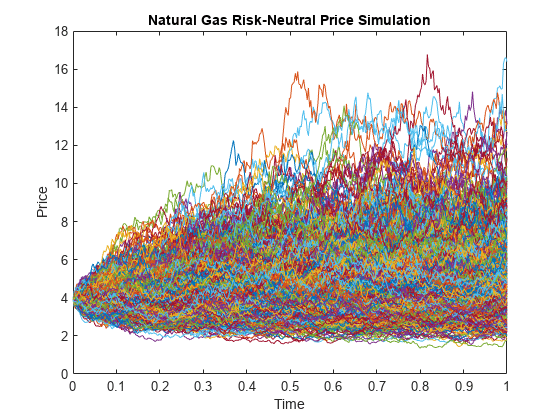
In this example, natural gas is used as the underlying asset with a mean-reverting dynamic. However, the Longstaff-Schwartz algorithm can be used for other underlying assets, such as electricity, with any underlying price dynamic.

Pricing the Swing Option

我们考虑与五摇摆摇摆的选择权利at the strike of $4.69/MMBtu, which can be exercised daily between the day after the settlement date and the maturity date. The Daily Contract Quantity (DCQ) is 10,000 MMBtu, which is the average amount of natural gas that the consumer expects to purchase on a given day. The consumer has the flexibility to reduce the purchase amount (downswing) in one day to the minimum DCQ of 2,500 MMBtu, or increase the purchase (upswing) to 15,000 MMBtu. The continuously compounded annual risk-free rate is 1%.

RateSpecis used to represent the interest-rate term structure. For the sake of simplicity, we consider a flat interest-rate term structure in this example. The values ofRateSpeccan be modified to accommodate any interest-rate curve. The functionhswingbylsin this example assumes a daily exercise if theExerciseDatesinput is empty.

% Define RateSpecrfrate = 0.01; Compounding = -1; RateSpec = intenvset('ValuationDate', Settle,'StartDates', Settle,...'EndDates', Maturity,'Rates', rfrate,...'Compounding', Compounding,'Basis', Basis);% Daily exercise% hswingbyls assumes daily exercise for empty ExerciseDatesExerciseDates = [];% Number of swingsNumSwings = 5;% Daily Contract Quantity in MMBtuDCQ = 10000;% Minimum DCQ constraint in MMBtuminDCQ = 2500;% Maximum DCQ constraint in MMBtumaxDCQ = 15000;% StrikeStrike = 4.69;

The Longstaff-Schwartz method is a backward iteration algorithm, which steps backward in time from the maturity date. At each exercise date, the algorithm approximates the continuation value, which is the value of the option if it is not exercised. This is done by fitting a regression against the values of the simulated prices and the discounted future value of the option at the next exercise date. The future value of the option is known as the algorithm moves backward in time. The continuation value is compared to the sum of the payoff from immediate exercise (a downswing or upswing) and the continuation value of a swing option with one less swing right. If this sum is smaller, the option holder's optimal strategy is to not exercise on that date. The functionhswingbylsin this example uses this method to determine the optimal exercise strategy and the price for swing options [1,2,7].

As discussed earlier, the only constraint considered in this example is the minimum and maximum DCQ. In this case, the optimal early exercise strategy is of a "bang-bang" type. This means that when it is optimal to upswing or downswing at a certain exercise date, the option holder should always exercise at the maximum or minimum DCQ to maximize profit. The "bang-bang" exercise would not be the optimal strategy if, for example, there is a terminal penalty based on volume. The pricing algorithm would then need to additionally keep track of all possible volume levels, which significantly adds to the runtime performance cost.

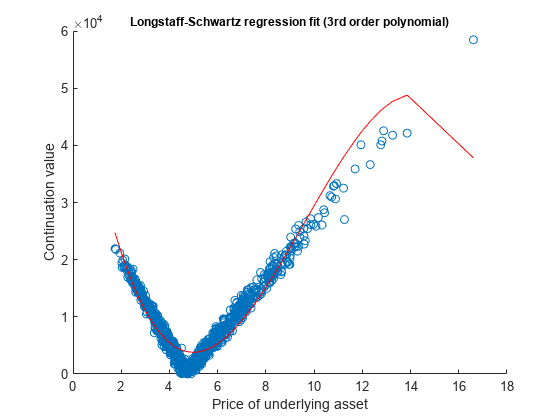
First, the swing option is priced using a third order polynomial to fit the regression of the Longstaff-Schwartz method. The functionhswingbylsalso generates a plot of the regression between the underlying price and the continuation value at the exercise date before maturity.

% Price swing option using 3rd order polynomial to fit Longstaff-Schwartz% regressiontic; useSpline = false; SwingPrice = hswingbyls(Paths, Times, RateSpec, Settle, Maturity,...Strike, ExerciseDates, NumSwings, DCQ, minDCQ, maxDCQ, useSpline,...[], true)

SwingPrice = 5.6943e+04

lsPolyTime = toc;

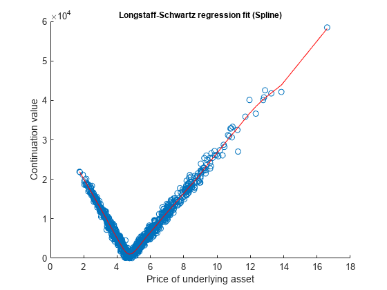
The above plot of the regression fit shows that the third order polynomial does not fit the continuation value perfectly, especially near the hinge and at the extreme points. Use thecsaps函数以适应使用立方斯穆特回归hing spline with a smoothing parameter of 0.7. The Curve Fitting Toolbox™ is required to run the remainder of the example.

% Price swing option using smoothed splines to fit Longstaff-Schwartz% regressiontic; useSpline = true; smoothingParam = 0.7; SwingPriceSpline = hswingbyls(Paths, Times, RateSpec, Settle, Maturity,...Strike, ExerciseDates, NumSwings, DCQ, minDCQ, maxDCQ, useSpline,...smoothingParam, true)

SwingPriceSpline = 6.0757e+04

lsSplineTime = toc;

The plot of the regression shows that the cubic smoothing spline has a better fit against the data, thus obtaining a more accurate value for the continuation values. However, the comparison below shows that using a cubic smoothing spline takes longer than a third order polynomial.

% Print comparison of running timesdisplayRunningTimes(lsPolyTime, lsSplineTime)

Comparison of running times: 3rd order polynomial: 9.13 sec Spline : 12.96 sec

Also, it is important to note that the price represents solely the optionality component. Hence, the price of the baseload forward contract is not included in the above calculated price. Because we used a fixed strike price, the baseload contract has a non-zero value, which can be calculated by:

where $$t_i,i=1,...,N,$$are the exercise dates (see [3] for more details). The full price of the contract, including the baseload and the swing option, is calculated below using the swing option price from the smoothed cubic spline.

% Obtain discount factorsRS2 = intenvset(RateSpec,'StartTimes', 0,'EndTimes', Times(2:end)); D = intenvget(RS2,'Disc');% Calculate baseload priceBaseLoadPrice = DCQ.*mean(Paths(2:end,:)-Strike,2)'*D;% Calculate full contract price, based on results from cubic spline LSFullContractPrice = BaseLoadPrice + SwingPriceSpline

FullContractPrice = 1.2482e+05

Price Bounds

A lower bound for the swing option is a strip of European options, and the upper bound is a strip of American options [4]. Compared to European options, swing options have an early exercise premium at each exercise date, thus the price should be higher. The price is lower than the American option strips, because only a single swing right can be exercised at each exercise date. More than one strip can be exercised in a single day using American options.

The prices for the strips of the lower and upper bounds are calculated below to check that the swing option prices are within these bounds. The European strip prices are calculated against the last five exercise dates.

% Obtain discount factor for the last NumSwings exercise datesD = D(end-NumSwings+1:end);% European lower boundidx = size(Paths, 1):-1:(size(Paths, 1) - NumSwings + 1); putEuro = D'*mean(max(Strike - Paths(idx,:), 0),2); callEuro = D'*mean(max(Paths(idx,:) - Strike, 0),2); lowerBound = ((DCQ-minDCQ).*putEuro+(maxDCQ-DCQ).*callEuro);% American upper bound[putAmer, callAmer] = hamericanPrice(Paths, Times, RateSpec, Strike); upperBound = NumSwings.*((DCQ-minDCQ).*putAmer+(maxDCQ-DCQ).*callAmer);% Print price and lower/upper boundsdisplaySummary(SwingPriceSpline, lowerBound, upperBound);

Comparison to lower and upper bounds: Lower bound (European) : 44412.14 Swing Option Price : 60757.33 Upper bound (American) : 68181.42

The prices calculated using the Longstaff-Schwartz algorithm are within the lower and upper bounds. The plot below shows a comparison between the swing option and the upper and lower bounds as the number of swings increases. When the number of swings is1, the swing option is equivalent to an American option. In the case of daily exercise opportunity (NumSwings = 365), the swing option is equivalent to the strip of European options with daily maturity.

Conclusion

The example shows the use of the Longstaff-Schwartz method to price a swing option where the underlying asset follows a mean-reverting dynamic. A 3rd order polynomial and a smoothed cubic spline are used to fit the regression in the Longstaff-Schwartz algorithm to approximate the continuation value. It was shown that the smoothed cubic spline fits the data better at the cost of slower performance. Finally, the resulting swing option prices were checked against the lower bound of a strip of European options and an upper bound of a strip of American options.

References

[1] Boogert, A., de Jong, C. "Gas Storage Valuation Using a Monte Carlo Method."Journal of Derivatives.15(3):81-98, 2008.

[2] Dorr, Uwe. "Valuation of Swing Options and Estimation of Exercise strategies by Monte Carlo Techniques." Oxford, 2002.

[3] Hull, John C.Options, Futures, and Other Derivatives. Sixth Edition, Pearson Education, Inc., 2006.

[4] Jaillet, P., Ronn, E. I., Tompaidis, S. "Valuation of Commodity-Based Swing Options,Management Science.50(7):909-921, 2004.

[5] Loland, Ambers, Lindqvist, Ola. "Valuation of Commodity-Based Swing Options: A Survey." Norsk, Regnesentral, 2008.

[6] Longstaff, Francis A., Schwartz, Eduardo S. "Valuing American Options by Simulation: A Simple Least-Squares Approach."The Review of Financial Studies.14(1):113-147, 2001.

[7] Meinshausen, N., Hambly, B.M. "Monte Carlo Methods for the Valuation of Multiple Exercise Options."Mathematical Science.14:557-583, 2004.

[8] Schwartz, Eduardo S. "The Stochastic Behavior of Commodity Prices: Implications for Valuation and Hedging."《金融杂志》上。52(3):923-973, 1997.

Utility Functions

functiondisplaySummary(SwingPriceSpline, lowerBound, upperBound) fprintf('Comparison to lower and upper bounds:\n'); fprintf('\n') fprintf('Lower bound (European) : %.2f\n', lowerBound); fprintf('Swing Option Price : %.2f\n', SwingPriceSpline); fprintf('Upper bound (American) : %.2f\n\n', upperBound);endfunctiondisplayRunningTimes(lsPolyTime, lsSplineTime) fprintf('Comparison of running times:\n'); fprintf('\n') fprintf('3rd order polynomial: %.2f sec\n', lsPolyTime); fprintf('Spline : %.2f sec\n\n', lsSplineTime);end