The Data Set

We start by looking at the data set SteamEng.

loadSteameng

This data set is collected from a laboratory scale steam engine. It has the inputs压力of the steam (actually compressed air) after the control valve, and磁化电压over the generator connected to the output axis.

The outputs are产生的电压in the generator andRotational speed发电机的（生成的交流电压的频率）。样品时间为50 ms。

First collect the measured channels into aniddata目的：

steam = iddata([GenVolt,Speed],[Pressure,MagVolt],0.05); steam.InputName = {'Pressure';'MagVolt'}; steam.OutputName = {'GenVolt';'Speed'};

Let us have a look at the data

plot(steam(:,1,1))

plot(steam(:,1,2))

plot(steam(:,2,1))

plot(steam(:,2,2))

Step and Impulse Responses

A first step to get a feel for the dynamics is to look at the step responses between the different channels estimated directly from data:

mi = impulseest(steam,50); clf, step(mi)

与信心区的回应

To look at the significance of the responses, the impulse plot can be used instead, with confidence regions corresponding to 3 standard deviations:

showconvidence（Impulseplot（MI），3）

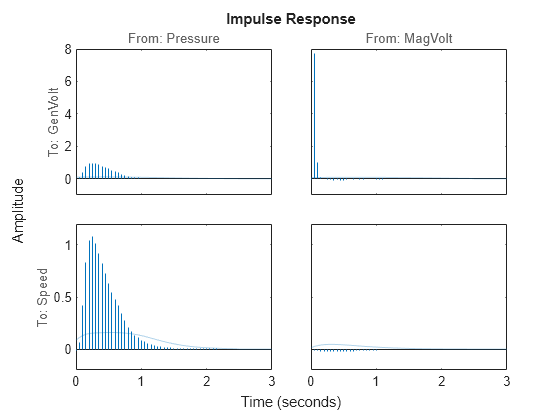
Clearly the off-diagonal influences dominate (Compare the y-scales!) That is,GenVoltis primarily affected byMagVolt(not much dynamics) andSpeedprimarily depends on压力. Apparently the response fromMagVolttoSpeed不是很重要。

A Two-Input-Two-Output Model

A quick first test is also to look a a default continuous time state-space prediction error model. Use only the first half of the data for estimation:

MP= ssest(steam(1:250))

mp =连续时间确定的状态空间模型：dx/dt = a x（t） + b u（t） + k e（t）y（t）= c x（t） + d u（t） + e（t） + e(t) A = x1 x2 x3 x4 x1 -29.43 -4.561 0.5994 -5.2 x2 0.4849 -0.8662 -4.101 -2.336 x3 2.839 5.084 -8.566 -3.855 x4 -12.13 0.9224 1.818 -34.29 B = Pressure MagVolt x1 0.1033 -1.617 x2 -0.3027-0.09415 X3 -1.566 0.2953 X4 -0.04477 -2.681 C = X1 X2 X2 X3 X4 GenVolt -16.39 0.3767 -0.7566 2.808 Speed -5.623 2.246 2.246 2.246 -0.5356 -0.5356 3.423 D = 0.50 0 0.0 SPEED 0 0 0.0 SPEED 0 0.0速度x = keps速度x =-0.02311 5.195 x3 1.526 2.132 x4 1.787 0.03216参数化：自由形式（A，B，C免费）。进料：无干扰部分：免费系数的估计数：40使用“ IDSSDATA”，“ GETPVEC”，“ GETCOV”，用于参数及其不确定性。状态：使用SST在时域数据进行估计。适合估计数据：[86.9; 74.84]％（预测焦点）FPE：3.897E-05，MSE：0.01414

与直接从数据估计的步骤响应进行比较：

h = stepplot(mi,'b',mp,'r',2);百分比蓝色用于直接估计，MP红色表演信号（h）

The agreement is good with the variation permissible within the shown confidence bounds.

To test the quality of the state-space model, simulate it on the part of data that was not used for estimation and compare the outputs:

compare(steam(251:450),mp)

The model is very good at reproducing the Generated Voltage for the validation data, and does a reasonable job also for the speed. (Use the pull-down menu to see the fits for the different outputs.)

Spectral Analysis

同样，比较的频率响应的比较MPwith a spectral analysis estimate gives:

msp = spa(steam);

bode(msp,mp)

CLF，Bode（MSP，'b',mp,'r')

You can right-click on the plot and select the different I/O pairs for close looks. You can also choose 'Characteristics: Confidence Region' for a picture of the reliability of the bode plot.

As before the response fromMagVolttoSpeedis insignificant and difficult to estimate.

Single-Input-Single-Output (SISO) Models

This data set quickly gave good models. Otherwise you often have to try out sub-models for certain channels, to see significant influences The toolbox objects give full support to the necessary bookkeeping in such work. The input and output names are central for this.

The step responses indicate thatMagVoltprimarily influencesGenVoltwhile压力primarily affectsSpeed. Build two simple SISO model for this: Both names and numbers can be used when selecting channels.

m1 = tfest(steam(1:250,'Speed','Pressure'），2,1）;% TF model with 2 poles 1 zerom2 = tfest（蒸汽（1：250,1,2），1,0）% Simple TF model with 1 pole.

m2 = From input "MagVolt" to output "GenVolt": 18.57 --------- s + 43.53 Continuous-time identified transfer function. Parameterization: Number of poles: 1 Number of zeros: 0 Number of free coefficients: 2 Use "tfdata", "getpvec", "getcov" for parameters and their uncertainties. Status: Estimated using TFEST on time domain data. Fit to estimation data: 73.34% FPE: 0.04645, MSE: 0.04535

Compare these models with the MIMO model mp:

compare(steam(251:450),m1,m2,mp)

The SISO models compare well with the full model. Let us now compare the Nyquist plots.m1is blue,m2is green andMPis red. Note that the sorting is automatic.MPdescribes all input output pairs, whilem1only contains压力toSpeed和m2only containsMagVolttoGenVolt.

clf showConfidence(nyquistplot(m1,'b'，m2，'g',mp,'r'),3)

The SISO models do a good job to reproduce their respective outputs.

The rule-of-thumb is that the model fitting becomes harder when you add more outputs (more to explain!) and simpler when you add more inputs.

两输入单一输出模型

To do a good job on the outputGenVolt, both inputs could be used.

m3 = armax（蒸汽（1：250，'GenVolt',:),'na'，4，'nb'，[4 4]，'NC',2,'nk'，[1 1]）;m4 = tfest（蒸汽（1：250，'GenVolt'，:)，2,1）;比较（Steam（251：450），MP，M3，M4，M2）

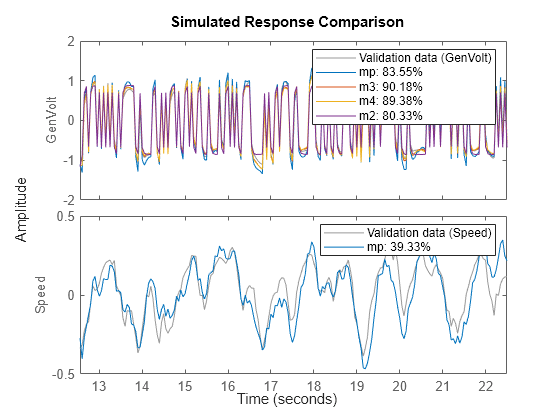
About 10% improvement was possible by including the input压力in the modelsm3(discrete time) andm4（连续时间），相比m2that uses justMagVoltas input.

Merging SISO Models

If desired, the two SISO modelsm1和m2can be put together as one "Off-Diagonal" model by first creating a zero dummy model:

mdum = idss(zeros(2,2),zeros(2,2),zeros(2,2),zeros(2,2)); mdum.InputName = steam.InputName; mdum.OutputName = steam.OutputName; mdum.ts = 0;％连续时间模型m12 = [idss(m1),mdum('Speed','MagVolt')];% Adding Inputs.来自两个输入到速度的％m22 = [mdum（mdum）（'GenVolt','Pressure'),idss(m2)];% Adding Inputs.% From both inputs to GenVolt毫米= [m12;m22];% Adding the outputs to a 2-by-2 model.compare(steam(251:450),mp,mm)

显然是“非对角线”模型毫米performs likem1和m2在解释输出时。