Structure From Motion From Two Views

Open Live Script

结构与运动(SfM) esti的过程mating the 3-D structure of a scene from a set of 2-D images. This example shows you how to estimate the poses of a calibrated camera from two images, reconstruct the 3-D structure of the scene up to an unknown scale factor, and then recover the actual scale factor by detecting an object of a known size.

Overview

This example shows how to reconstruct a 3-D scene from a pair of 2-D images taken with a camera calibrated using theCamera Calibratorapp. The algorithm consists of the following steps:

Match a sparse set of points between the two images. There are multiple ways of finding point correspondences between two images. This example detects corners in the first image using thedetectMinEigenFeaturesfunction, and tracks them into the second image usingvision.PointTracker. Alternatively you can useextractFeaturesfollowed bymatchFeatures.
Estimate the fundamental matrix usingestimateEssentialMatrix.
Compute the motion of the camera using therelativeCameraPosefunction.
Match a dense set of points between the two images. Re-detect the point usingdetectMinEigenFeatureswith a reduced'MinQuality'to get more points. Then track the dense points into the second image usingvision.PointTracker.
Determine the 3-D locations of the matched points usingtriangulate.
Detect an object of a known size. In this scene there is a globe, whose radius is known to be 10cm. Usepcfitsphereto find the globe in the point cloud.
Recover the actual scale, resulting in a metric reconstruction.

Read a Pair of Images

Load a pair of images into the workspace.

imageDir = fullfile(toolboxdir('vision'),'visiondata','upToScaleReconstructionImages'); images = imageDatastore(imageDir); I1 = readimage(images, 1); I2 = readimage(images, 2); figure imshowpair(I1, I2,'montage'); title(“阿riginal Images');

Figure contains an axes object. The axes object with title Original Images contains an object of type image.

Load Camera Parameters

This example uses the camera parameters calculated by theCamera Calibratorapp. The parameters are stored in thecameraParamsobject, and include the camera intrinsics and lens distortion coefficients.

% Load precomputed camera parametersloadupToScaleReconstructionCameraParameters.mat

Remove Lens Distortion

Lens distortion can affect the accuracy of the final reconstruction. You can remove the distortion from each of the images using theundistortImagefunction. This process straightens the lines that are bent by the radial distortion of the lens.

I1 = undistortImage(I1, cameraParams); I2 = undistortImage(I2, cameraParams); figure imshowpair(I1, I2,'montage'); title('Undistorted Images');

Figure contains an axes object. The axes object with title Undistorted Images contains an object of type image.

Find Point Correspondences Between The Images

Detect good features to track. Reduce'MinQuality'to detect fewer points, which would be more uniformly distributed throughout the image. If the motion of the camera is not very large, then tracking using the KLT algorithm is a good way to establish point correspondences.

% Detect feature pointsimagePoints1 = detectMinEigenFeatures(im2gray(I1),'MinQuality', 0.1);% Visualize detected pointsfigure imshow(I1,'InitialMagnification', 50); title('150 Strongest Corners from the First Image'); holdonplot(selectStrongest(imagePoints1, 150));

Figure contains an axes object. The axes object with title 150 Strongest Corners from the First Image contains 2 objects of type image, line.

% Create the point trackertracker = vision.PointTracker('MaxBidirectionalError', 1,'NumPyramidLevels', 5);% Initialize the point trackerimagePoints1 = imagePoints1.Location; initialize(tracker, imagePoints1, I1);% Track the points[imagePoints2, validIdx] = step(tracker, I2); matchedPoints1 = imagePoints1(validIdx, :); matchedPoints2 = imagePoints2(validIdx, :);% Visualize correspondencesfigure showMatchedFeatures(I1, I2, matchedPoints1, matchedPoints2); title('Tracked Features');

Figure contains an axes object. The axes object with title Tracked Features contains 4 objects of type image, line.

Estimate the Essential Matrix

Use theestimateEssentialMatrixfunction to compute the essential matrix and find the inlier points that meet the epipolar constraint.

% Estimate the fundamental matrix[E, epipolarInliers] = estimateEssentialMatrix(...matchedPoints1, matchedPoints2, cameraParams,'Confidence', 99.99);% Find epipolar inliersinlierPoints1 = matchedPoints1(epipolarInliers, :); inlierPoints2 = matchedPoints2(epipolarInliers, :);% Display inlier matchesfigure showMatchedFeatures(I1, I2, inlierPoints1, inlierPoints2); title('Epipolar Inliers');

Figure contains an axes object. The axes object with title Epipolar Inliers contains 4 objects of type image, line.

Compute the Camera Pose

Compute the location and orientation of the second camera relative to the first one. Note thattis a translation unit vector, because translation can only be computed up to scale.

[orient, loc] = relativeCameraPose(E, cameraParams, inlierPoints1, inlierPoints2);

Reconstruct the 3-D Locations of Matched Points

Re-detect points in the first image using lower'MinQuality'to get more points. Track the new points into the second image. Estimate the 3-D locations corresponding to the matched points using thetriangulatefunction, which implements the Direct Linear Transformation (DLT) algorithm [1]. Place the origin at the optical center of the camera corresponding to the first image.

% Detect dense feature points. Use an ROI to exclude points close to the% image edges.roi = [30, 30, size(I1, 2) - 30, size(I1, 1) - 30]; imagePoints1 = detectMinEigenFeatures(im2gray(I1),'ROI', roi,...'MinQuality', 0.001);% Create the point trackertracker = vision.PointTracker('MaxBidirectionalError', 1,'NumPyramidLevels', 5);% Initialize the point trackerimagePoints1 = imagePoints1.Location; initialize(tracker, imagePoints1, I1);% Track the points[imagePoints2, validIdx] = step(tracker, I2); matchedPoints1 = imagePoints1(validIdx, :); matchedPoints2 = imagePoints2(validIdx, :);% Compute the camera matrices for each position of the camera% The first camera is at the origin looking along the Z-axis. Thus, its% transformation is identity.tform1 = rigid3d; camMatrix1 = cameraMatrix(cameraParams, tform1);% Compute extrinsics of the second camera东方cameraPose = rigid3d (loc);tform2 = cameraPoseToExtrinsics(cameraPose); camMatrix2 = cameraMatrix(cameraParams, tform2);% Compute the 3-D pointspoints3D = triangulate(matchedPoints1, matchedPoints2, camMatrix1, camMatrix2);% Get the color of each reconstructed pointnumPixels = size(I1, 1) * size(I1, 2); allColors = reshape(I1, [numPixels, 3]); colorIdx = sub2ind([size(I1, 1), size(I1, 2)], round(matchedPoints1(:,2)),...round(matchedPoints1(:, 1))); color = allColors(colorIdx, :);% Create the point cloudptCloud = pointCloud(points3D,'Color', color);

Display the 3-D Point Cloud

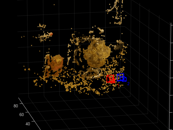
Use theplotCamerafunction to visualize the locations and orientations of the camera, and thepcshowfunction to visualize the point cloud.

% Visualize the camera locations and orientationscameraSize = 0.3; figure plotCamera('Size', cameraSize,'Color','r','Label','1',“阿pacity', 0); holdongridonplotCamera('Location', loc,“阿rientation', orient,'Size', cameraSize,...'Color','b','Label','2',“阿pacity', 0);% Visualize the point cloudpcshow(ptCloud,'VerticalAxis','y','VerticalAxisDir','down',...'MarkerSize', 45);% Rotate and zoom the plotcamorbit(0, -30); camzoom(1.5);%标签轴xlabel('x-axis'); ylabel('y-axis'); zlabel('z-axis') title('Up to Scale Reconstruction of the Scene');

Figure contains an axes object. The axes object with title Up to Scale Reconstruction of the Scene contains 21 objects of type line, text, patch, scatter.

Fit a Sphere to the Point Cloud to Find the Globe

Find the globe in the point cloud by fitting a sphere to the 3-D points using thepcfitspherefunction.

% Detect the globeglobe = pcfitsphere(ptCloud, 0.1);% Display the surface of the globeplot(globe); title('Estimated Location and Size of the Globe'); holdoff

Figure contains an axes object. The axes object with title Estimated Location and Size of the Globe contains 22 objects of type line, text, patch, scatter, surface.

Metric Reconstruction of the Scene

The actual radius of the globe is 10cm. You can now determine the coordinates of the 3-D points in centimeters.

% Determine the scale factorscaleFactor = 10 / globe.Radius;% Scale the point cloudptCloud = pointCloud(points3D * scaleFactor,'Color', color); loc = loc * scaleFactor;% Visualize the point cloud in centimeterscameraSize = 2; figure plotCamera('Size', cameraSize,'Color','r','Label','1',“阿pacity', 0); holdongridonplotCamera('Location', loc,“阿rientation', orient,'Size', cameraSize,...'Color','b','Label','2',“阿pacity', 0);% Visualize the point cloudpcshow(ptCloud,'VerticalAxis','y','VerticalAxisDir','down',...'MarkerSize', 45); camorbit(0, -30); camzoom(1.5);%标签轴xlabel('x-axis (cm)'); ylabel('y-axis (cm)'); zlabel('z-axis (cm)') title('Metric Reconstruction of the Scene');

Figure contains an axes object. The axes object with title Metric Reconstruction of the Scene contains 21 objects of type line, text, patch, scatter.

Summary

This example showed how to recover camera motion and reconstruct the 3-D structure of a scene from two images taken with a calibrated camera.

References

[1] Hartley, Richard, and Andrew Zisserman. Multiple View Geometry in Computer Vision. Second Edition. Cambridge, 2000.