在这个视频中,我们将看到之前学过的小波概念的实际应用。我将说明如何使用连续小波变换对信号进行良好的时频分析。首先,让我们在MATLAB中加载一个地震信号。此信号以1hz采样,持续51分钟。您可以使用plot命令查看信号。观察信号的时域表示,我们看到两个不同的区域。第一次地震活动发生在30分钟左右。这只持续很短的时间。第二次地震活动发生在大约34分钟左右,时间相对较长。你可以看到,仅仅通过观察时域表示就很难将噪声从地震信号中分离出来。 Many naturally occurring signals have similar characteristics. They are composed of slowly varying components interspersed with abrupt changes and are often buried in noise. Wavelets are very useful in analyzing these kinds of signals. We will see how a bit later. But first, let us see what happens when we use the short time Fourier transform to produce a time-frequency visualization. We pass in the signal and the sampling frequency as input arguments to the function spectrogram. Looking at the output, you can see that the two instances of seismic activity we just saw are now indistinguishable. All we see is a signal whose frequency is spread around 0.05 Hz but is not very well localized. Let us see what happens when we try to localize the events by reducing the window size used in the spectrogram. By reducing the size of the window, we see some bright spots around 30 and 33 mins, but the two events are not well separated. The frequency and time uncertainty of the events is still very high. Reducing the window size was not very helpful. We need to somehow localize the frequency information of these two events. Now let us repeat the analysis - this time using wavelets. We will use the CWT function in MATLAB to compute the Continuous Wavelet Transform. This will help obtain a joint time frequency analysis of the earthquake data. The CWT function supports these analytic key wavelets. If you don’t specify which wavelet you want to use, the CWT uses morse wavelets by default. When no output parameters are specified, the function, CWT produces a joint time -frequency visualization of the input signal. The minimum and maximum scales for analysis are determined automatically by the CWT function based on the wavelet's energy spread. The magnitude of the wavelet coefficients returned by the function are color coded. The white dashed lines denote the cone of influence. Within this region, the wavelet coefficient estimates are reliable. Looking at the plot, we can see the two regions produced by the earthquake. The first seismic activity is clearly separated from the second. Both these events seem to be well localized in time and frequency. For a richer time-frequency analysis, you can choose to vary the wavelet scales over which you want to carry out the analysis. You can do this by using different parameters. For this example, we will set the number of octaves to 10 and the number of voices per octave to 32. The function returns the wavelet coefficients and the equivalent frequencies as outputs. We can plot the coefficients a as function of time and frequency plot, using the surface command. Looking at this plot, it is clear that the frequency of the seismic event ranges from 0.03 Hz to 0.06 Hz. We can also reconstruct the time-domain representation of this seismic event from the wavelet coefficients using the function icwt. We pass in the wavelet coefficients and the frequency vector, which is the output of the CWT function. We also pass the frequency range of the signal that we want to extract. In this case, we’re inputting 0.03 to 0.06. The output is a time-domain representation of the seismic signal of interest. This way, you can use wavelets for performing joint time-frequency analysis.