Today, I'd like to welcome Josh Meyer as this week's guest blogger. Josh works on the Documentation team here at MathWorks, where he writes and maintains some of the MATLAB Mathematics documentation. In this post, Josh provides a bit of advice on how to choose which ODE solver to use. Over to you, Josh...

Contents

Initial Value Problems

There are 7 ordinary differential equation initial value problem solvers in MATLAB:

(note thatode15i剩下的讨论,因为它解决了吗ts own class of initial value problems: fully implicit ODEs of the form $f(t,y,y') = 0$)

To choose between the solvers, it's first necessary to understand why one solver might be better than another for a given problem.

The ODE solvers in MATLAB all work on initial value problems of the form,

$$y' = f \left( t,y \right)$$

where $y' = dy/dt$. There is also a more general form,

$$ M(t,y) y' = f \left( t,y \right)$$

where $M(t,y)$ is referred to as the质量矩阵.

Starting with the initial conditions $y_0$, and a period of time over which the answer is to be obtained $(t_0,t_f)$, the solution is obtained iteratively by using the results of previous steps according to the solver's algorithm. At the first such step, the initial conditions provide the necessary information that allows the integration to proceed. The final result is that the ODE solver returns a vector of time steps $t_0,t_1,...,t_f$ as well as the corresponding solution at each time step $y_0,y_1,...,y_f$.

Theoretically, this numerical solution technique is possible because of the connection between differential equations and integrals provided by the fundamental theorem of calculus:

$$y(t + h) = y(t) + \int_t^{t+h} f\left( s,y(s) \right) ds$$

The problem of calculating $y(t+h)$ becomes a question of how to approximate the integral on the right hand side. This is where different solvers come in. Each different solver evaluates the integral using different numerical techniques, and each solver makes trade-offs between efficiency and accuracy.

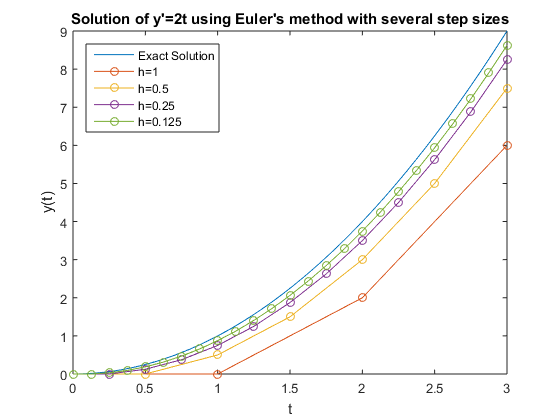
Example: Euler's Method

Euler's method is a simple ODE solver, but it provides an illustration of the trade-offs between efficiency and accuracy in an ODE solver algorithm. Suppose you want to solve

$$y' = f(t,y) = 2t$$

over the time span $[0,3]$ using the initial condition $y_0 = 0$. Each step of Euler's method is computed with

$$\begin{array}{cl} y_{n+1} &= y_n + h f \left(t_n,y_n\right)\\ t_{n+1}&= t_n + h\end{array}$$

Using $h=1$, the solution requires just three steps:

$$\begin{array}{cl} y_1 &= y_0 + f\left(t_0,y_0\right)=0\\y_2 &= y_1 + f\left(t_1,y_1 \right)=2\\y_3 &= y_2 + f\left(t_2,y_2 \right)=6 \end{array}$$

... But is it accurate?

Not really. The exact solution to this equation is

$$y(t) = t^2$$

Reducing the step size $h$ can improve the accuracy of the answer a bit, but it also requires more steps to achieve the solution. To see this, the below code solves this problem using Euler's method and compares the answer to the analytic solution for several different values of $h$.

clear, clc h = 1; tspan = [0 3]; f = @(t,y) 2*t; dydt(1) = 0; t(1) = 0; y = @(t) t.^2; x = linspace(0,tspan(end)); figure plot(x,y(x)) xlabel('t'), ylabel('y(t)') holdonwhileh > 0.1fork = 2:tspan(end)/h+1 dydt(k) = dydt(k-1) + h*f(t(k-1),dydt(k-1)); t(k) = t(k-1) + h;endplot(t,dydt,'-o') h = h/2;endlegend('Exact Solution',“h = 1”,'h=0.5','h=0.25','h=0.125',...'Location','NorthWest') title('Solution of y''=2t using Euler''s method with several step sizes')

Improving on Euler's Method

Using smaller and smaller step sizes turns out to not be a good idea, since the algorithm loses efficiency. For any reasonable problem such a solver would be very slow. Also, Euler's method has a few inherent problems. Since the slope of $y$ is evaluated only once at the beginning of each interval, this solver only produces exact answers for constant functions. There is also no way to estimate the error, so the solver needs to use fixed step sizes.

So, one way to improve on Euler's method is to evaluate $y'$ more often in each step. This provides intermediate slopes that give a better idea of what the function is doing within each interval, allowing the solver to produce exact answers for higher order problems. For example, if you add an evaluation of the slope halfway across each interval to Euler's method, then the result is called themidpoint rule, which produces exact integrations for linear functions:

$$\begin{array}{cl} s_1 &= f(t_n,y_n)\\ s_2 &= f\left( t_n + \frac{h}{2}, y_n + \frac{h}{2}s_1\right)\\y_{n+1} &= y_n + hs_2\\t_{n+1} &= t_n+h\end{array}$$

If you evaluate the slope four times in each interval, you get theclassical Runge-Kuttaalgorithm (a.k.a.RK4), which is a piece of theode45算法。该算法产生的确切integrations for cubic functions (and if $f$ is only a function of $t$, then $s_2=s_3$ and this is the same asSimpson's rulefor quadrature):

$$\begin{array}{cl} s_1 &= f(t_n,y_n)\\s_2 &= f\left(t_n+\frac{h}{2},y_n+\frac{h}{2}s_1\right)\\s_3 &= f\left(t_n+\frac{h}{2},y_n+\frac{h}{2}s_2\right)\\ s_4 &= f\left(t_n+h,y_n+hs_3\right)\\y_{n+1} &= y_n + \frac{h}{6}\left(s_1+2s_2+2s_3+s_4\right)\\t_{n+1} &= t_n + h\end{array}$$

Runge-Kutta algorithms are allsingle-stepsolvers, since each step only depends on the result of the previous step.ode45,ode23,ode23s,ode23t, andode23tball employ single-step algorithms. Multi-step algorithms, such as those employed byode113andode15s, use the results of several past steps.

Sophisticated ODE solvers, like the ones in MATLAB, also estimate the error in each step to determine how big the next step size should be. This is another improvement over the fixed step sizes used above, since a solver that does more work per step is able to compensate by taking steps of varying size. The error estimate used to determine the step size is typically obtained by comparing the results of two different methods. MATLAB's ODE solvers follow a naming convention that reveals information about which methods they use.ode45compares the results of a 4th-order Runge-Kutta method and a 5th-order Runge-Kutta method to determine the error. Similarly,ode23uses a 2nd-order and 3rd-order Runge-Kutta comparison. So, in general, the smaller the numberodeNN, the looser the solver's error tolerance is.

It should be no surprise, then, thatode45obtains a very accurate answer for the equation we solved before with Euler's method.ode45is MATLAB's general purpose ODE solver, and it is the first solver you should use for most problems.

y = @(t) t.^2; x = linspace(0,3); figure plot(x,y(x)) xlabel('t'), ylabel('y(t)') holdon[t,y] = ode45(@(t,y) 2*t, [0 3], 0); plot(t,y,'o') xlabel('t'), ylabel('y(t)') title('Solution of y''=2t using ode45')

Stiff Differential Equations

For some ODE problems, the step size taken by the solver is forced down to an unreasonably small level in comparison to the interval of integration, even in a region where the solution curve is smooth. These step sizes can be so small that traversing a short time interval might require millions of evaluations. This can lead to the solver failing the integration, but even if it succeeds it will take a very long time to do so.

Equations that cause this behavior in ODE solvers are said to bestiff. This is a nod to the fact that the equations are stubborn and not easily evaluated with numerical techniques. The problem that stiff ODEs pose is that explicit solvers (such asode45) are untenably slow in achieving a solution. This is whyode45is classified as a nonstiff solver along withode23andode113. These solvers all struggle to integrate stiff equations.

Equation stiffness resists a precise definition, because there are several factors that cause it. Stiffness results from a combination of the specific equations, the ODE solver being used, the initial conditions, and the error tolerance used by the solver. The following statements about stiffness, attributed to Lambert [6], are exhibited by many examples of stiff ODEs, but counterexamples also exist, so they are not true definitions of stiffness:

A common theme among these statements is that stiffness can result from a difference in scaling somewhere in the problem. This difference in scale (for example, if the Jacobian $J = \partial f_n/\partial y_i$ has a large ratio of negative eigenvalues) constrains the step size that the solver can take in performing the integration. Tiny step sizes become necessary in order to preserve any notion of error tolerance or stability in the solution.

For example, equations describing chemical reactions frequently display stiffness, since it is common for components of the solution to vary on drastically different time scales (reactions occurring at the same time that are both very slow and very fast).

However, there are solvers specifically designed to work on stiff ODEs. Solvers that are designed for stiff problems typically do more work per step, and the pay-off is that they are able to take much larger steps and enjoy improved numerical stability compared to the nonstiff solvers. Stiff solvers are implicit, because the computation of $y$ requires the use of linear algebra to solve systems of linear equations. The Jacobian is used to estimate the local behavior of the ODE as the integration proceeds, so supplying the analytical Jacobian can improve the performance of MATLAB's stiff ODE solvers.

This is just a cursory treatment of stiffness, because it is a complex topic. SeeOrdinary Differential Equations: Stiffnessfor a more in-depth look.

To summarize, the nonstiff solvers in MATLAB are:

The stiff solvers are (whenode45is slow):

It should be noted that nonstiff solvers doworkon stiff problems, it is just that they are exceptionally slow. Similarly, solvers designed for stiff problems can work on nonstiff problems, but since they do more work per step they are less efficient than their nonstiff counterparts when that extra work isn't necessary. So equation stiffness is a matter of solver efficiency, and the goal is to strike the right balance between accuracy of the solution and work done in each step by the solver.

Solver Recommendations

The following recommendations are adapted from theMATLAB Mathematics documentation:

Fornonstiffproblems:

Forstiffproblems (whereode45is slow):

Here is a graphic that captures the basic recommendations. In most cases, the only choice in solver you will need to make is to useode15sinstead ofode45.

Example 1: Damped Pendulum

The equation of motion for a damped pendulum is,

$$\ddot{\theta} = -\frac{b}{m}\dot{\theta}-\frac{mg}{L\left(m-2b\right)} \sin \theta$$

g是美元引力常数,m m美元吗ass of the bob, $L$ the length of the string, and $b$ is a damping coefficient. The goal is to solve for $\theta$, the angle that the pendulum deviates from the vertical, and $\theta '$, the rate at which the angle changes.

Some natural initial conditions would be $\theta_0 = \pi/4$ and $\theta '_0 = 0$, indicating that you lift the pendulum up to a 45 degree angle before letting go, and it has no initial angular velocity. Due to the damping coefficient, you would expect the pendulum to slowly lose momentum and go back down to rest.

The filependulumODE.mreformulates the problem as a coupled system of first-order ODEs:

$$\begin{array}{cl} y_1' &= y_2\\y_2' &= -\frac{b}{m} y_2 -\frac{mg}{L(m-2b)}sin(y_1)\end{array}$$

then solves usingode45,ode15s,ode23, andode113. The solutions for $y_1 = \theta$ are plotted, and the file returns the stats for each solver. As is always the case when displaying execution times, "the timings displayed can vary".

functionpendulumODE opts = odeset('stats','on'); tspan = [0 25]; y0 = [pi/4, 0]; disp(' '), disp('Stats for ode45:') tic, [t1,y1] = ode45(@pendode, tspan, y0, opts); toc disp(' '), disp('Stats for ode15s:') tic, [t2,y2] = ode15s(@pendode, tspan, y0, opts); toc disp(' '), disp('Stats for ode23:') tic, [t3,y3] = ode23(@pendode, tspan, y0, opts); toc disp(' '), disp('Stats for ode113:') tic, [t4,y4] = ode113(@pendode, tspan, y0, opts); toc figure subplot(2,2,1), plot(t1,y1(:,1),'-o'), xlim([0 25]), title('ode45') subplot(2,2,2), plot(t2,y2(:,1),'-o'), xlim([0 25]), title('ode15s') subplot(2,2,3), plot(t3,y3(:,1),'-o'), xlim([0 25]), title('ode23') subplot(2,2,4), plot(t4,y4(:,1),'-o'), xlim([0 25]), title('ode113')functiondy2dt2 = pendode(t,y) g = 9.8;%m/s^2m = 1;% Mass of bobL = 2;% Length of pendulum in metersb = 0.2;% Damping coefficientdy2dt2 = [y(2); -b/m*y(2)-g/L*sin(y(1))];endend

pendulumODE

Stats for ode45: 75 successful steps 0 failed attempts 451 function evaluations Elapsed time is 0.011970 seconds. Stats for ode15s: 183 successful steps 9 failed attempts 315 function evaluations 1 partial derivatives 31 LU decompositions 311 solutions of linear systems Elapsed time is 0.081467 seconds. Stats for ode23: 263 successful steps 36 failed attempts 898 function evaluations Elapsed time is 0.015948 seconds. Stats for ode113: 159 successful steps 3 failed attempts 322 function evaluations Elapsed time is 0.018056 seconds.

The solvers all perform well, but the damped pendulum is a good example of a nonstiff problem whereode45performs nicely. In this caseode15sneeds to do extra work in order to achieve an inferior solution.

Example 2: van der Pol Oscillator

The van der Pol Oscillator equation becomes stiff in certain intervals when the nonlinear parameter $\mu$ is large:

$$\ddot{y} - \mu \left(1-y^2\right)\dot{y}+y=0$$

The nonlinearity of this equation is contained entirely in the term that involves $\mu$: notice that if $\mu=0$, the equation reduces to that of a simple harmonic oscillator, which has regular periodic behavior.

Attempting to solve this equation usingode45is met with severe resistance, requiring millions of evaluations and 30+ minutes of execution (I stopped execution after 35 minutes). Since the problem is clearly stiff, this example compares the stiff solvers.

The filevanderpolODE.mfinds the solution for $\mu=1000$ usingode15s,ode23s,ode23t, andode23tb. The function filevdp1000.mships with MATLAB and encodes this equation as a coupled system of first-order ODEs:

$$\begin{array}{cl}y_1' &= y_2\\y_2' &= \mu \left( 1-y_1^2 \right)y_2 - y_1\end{array}$$

The Jacobian is supplied to assist the solvers, and its use is reflected in the number of partial derivative evaluations.

functionvanderpolODE opts = odeset('stats','on','Jacobian',@J); tspan = [0 3000]; y0 = [2 0]; disp(' '), disp('Stats for ode15s:') tic, [t1,y1] = ode15s(@vdp1000, tspan, y0, opts); toc disp(' '), disp('Stats for ode23s:') tic, [t2,y2] = ode23s(@vdp1000, tspan, y0, opts); toc disp(' '), disp('Stats for ode23t:') tic, [t3,y3] = ode23t(@vdp1000, tspan, y0, opts); toc disp(' '), disp('Stats for ode23tb:') tic, [t4,y4] = ode23tb(@vdp1000, tspan, y0, opts); toc figure subplot(2,2,1), plot(t1,y1(:,1),'-o'), ylim([-4 4]), title('ode15s') subplot(2,2,2), plot(t2,y2(:,1),'-o'), title('ode23s') subplot(2,2,3), plot(t3,y3(:,1),'-o'), title('ode23t') subplot(2,2,4), plot(t4,y4(:,1),'-o'), title('ode23tb')functiondfdy = J(t,y) MU = 1000;% Nonlinear coefficientdfdy = [ 0 1 -2*MU*y(1)*y(2)-1 MU*(1-y(1)^2) ];endend

vanderpolODE

Stats for ode15s: 591 successful steps 225 failed attempts 1749 function evaluations 45 partial derivatives 289 LU decompositions 1747 solutions of linear systems Elapsed time is 0.192955 seconds. Stats for ode23s: 741 successful steps 13 failed attempts 2251 function evaluations 741 partial derivatives 754 LU decompositions 2262 solutions of linear systems Elapsed time is 0.092824 seconds. Stats for ode23t: 776 successful steps 94 failed attempts 2014 function evaluations 36 partial derivatives 294 LU decompositions 2012 solutions of linear systems Elapsed time is 0.218996 seconds. Stats for ode23tb: 573 successful steps 93 failed attempts 2816 function evaluations 44 partial derivatives 269 LU decompositions 3415 solutions of linear systems Elapsed time is 0.202237 seconds.

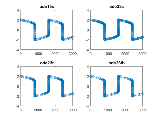
The plots are of the solutions for $y_1$. For this problem,ode23sexecutes quickest and with the least number of failed steps. The supplied Jacobian greatly assistsode23sin evaluating the partial derivatives in each step.ode23tbalso solves the problem with the fewest number of steps, outperformingode15s. This problem is a good example of a stiff problem with a crude tolerance whereode23sandode23tbcan out performode15s. But practically speaking, all of the stiff solvers perform well on this problem and offer significant time savings when compared toode45.

Summary

Although all of the ODE solvers are capable of working on the same problems, it's recommended that you start withode45. Then, if the problem exhibits signs of stiffness,ode15sis a good second choice. The other solvers then offer further refinement based on the properties of the specific problem and whether extra information (such as the Jacobian) can be provided.

Comments

Does your work involve the use of MATLAB's ODE solvers? If so, share your experiencehere.

Further Reading

[1] C. Moler,Ordinary Differential EquationsNumerical Computing with MATLABElectronic edition: The MathWorks, Inc., Natick, MA, 2004

[2] Shampine, L. F. and M. W. Reichelt,The MATLAB ODE SuiteSIAM Journal on Scientific Computing, Vol. 18, 1997.

[3] C. Moler,Ordinary Differential Equations: StiffnessCleve’s Corner: Cleve Moler on Mathematics and Computing, 2014

[4] L. F. Shampine,Numerical Solution of Ordinary Differential Equations, Chapman & Hall, 1994

[5] Shampine, L. F., Gladwell, I. and S. Thompson,Solving ODEs with MATLAB, Cambridge University Press, 2003

[6] J. D. Lambert,Numerical Methods for Ordinary Differential Systems, New York: Wiley, 1992

Copyright 2015 The MathWorks, Inc.

Get the MATLAB code

Published with MATLAB® R2015a