 Cleve’s Corner: Cleve Moler on Mathematics and Computing
 Loren on the Art of MATLAB
 Steve on Image Processing with MATLAB
 Guy on Simulink
 Deep Learning
 Developer Zone
 Stuart’s MATLAB Videos
 Behind the Headlines
 File Exchange Pick of the Week
 Hans on IoT
 Student Lounge
 Startups, Accelerators, & Entrepreneurs
 MATLAB Community
 MATLAB ユーザーコミュニティー
Plotting a* and b* colors
Today's blog post comes from planning one topic, but then taking a sharp left turn and doing something else completely. I was thinking about writing something related to
meshgrid
, and so I was looking at some old blog posts in which
meshgrid
was used. For example,
meshgrid
was used in this
30-Dec-2010 post
about the a* and b* component in the Lab color space.
In reading over that old post, however, I realized that I made a rather egregious conceptual error in it. I plotted colors over the domain
$ -100 \leq a^* \leq 100 $
,
$ -100 \leq b^* \leq 100 $
, using
$ L^* = 90 $
, without realizing or explaining that most of those
$ (L^*,a^*,b^*) $
combinations are far out of the sRGB gamut. In other words, they are not really displayable (even on a wide-gamut monitor). Also, the functions I used back then have since been superseded by new functions that are not only easier to use, but are also more helpful at looking at in-gamut vs. out-of-gamut questions.
I decided, therefore, to update and improve that old post.
Showing$ (a^*,b^*) $colors for a fixed$ L^* $
As I did last time, I'll start with
$ L^*=90 $
, which is at the bright end of the scale. For that choice of
$ L^* $
, let's see what the colors in the
$ (a^*,b^*) $
plane look like, taking into account colors that might be out of gamut.
clear
closeall
a = -110:0.4:110;
b = -110:0.4:110;
[aa,bb] = meshgrid(a,b);
L = 90;
LL = L*ones(size(aa));
lab = cat(3,LL,aa,bb);
In the old post, I used
makecform
and
applycform
to convert Lab values to sRGB values. This time, I'll use
lab2rgb
.
rgb = lab2rgb(lab);
When using
lab2rgb
, out-of-gamut values are indicated by output values that are greater than 1 or less than 0.
out_gamut_mask = any((rgb > 1) | (rgb < 0),3);
Let's replace the out-of-gamut colors with gray and display the result. Set the
y
方向的图像显示
“正常”
so that positive
$ b^* $
is at the top, which is the usual convention for these kinds of plots. Also, display the axes ticks and labels.
rgb(repmat(out_gamut_mask,1,1,3)) = 0.6;
imshow(rgb,'XData',b,'YData',a)
axisxy
axison
xlabel('$a^*$','Interpreter','latex')
ylabel('$b^*$','Interpreter','latex')
title('$L^*=90$','Interpreter','latex')
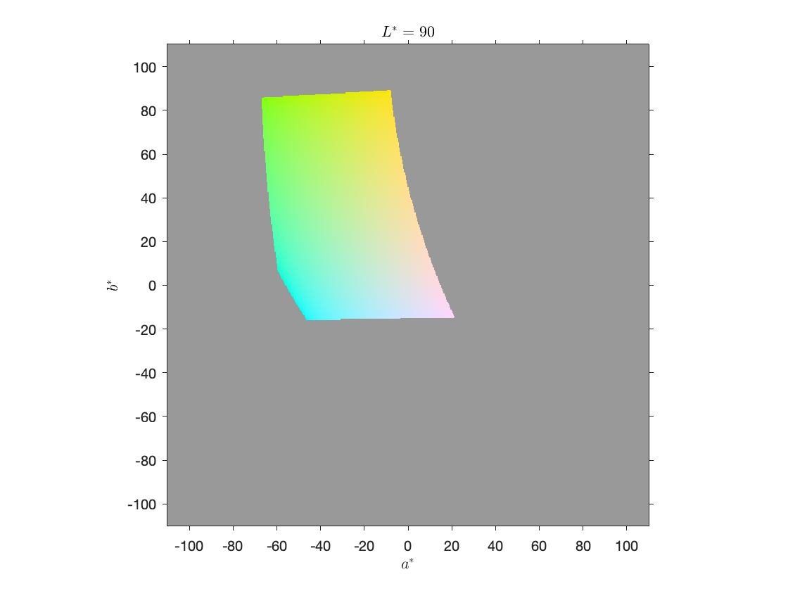
As you can see, with
$ L^*=90 $
, only a relatively small portion of the
$ (a^*,b^*) $
plane is in gamut.
Yellow is the brightest color
Let's repeat that process with an even brighter
$ L^* $
value, almost all the way to white.
L = 96;
LL = L*ones(size(aa));
lab = cat(3,LL,aa,bb);
rgb = lab2rgb(lab);
out_gamut_mask = any((rgb > 1) | (rgb < 0),3);
rgb(repmat(out_gamut_mask,1,1,3)) = 0.6;
imshow(rgb,'XData',b,'YData',a)
axisxy
axison
xlabel('$a^*$','Interpreter','latex')
ylabel('$b^*$','Interpreter','latex')
title('$L^*=96$','Interpreter','latex')
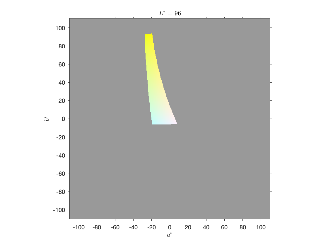
The plot above demonstrates that yellow is the only color that can be displayed almost as bright as white.
Blue is the darkest color
Now let's try something dark.
L = 25;
LL = L*ones(size(aa));
lab = cat(3,LL,aa,bb);
rgb = lab2rgb(lab);
out_gamut_mask = any((rgb > 1) | (rgb < 0),3);
rgb(repmat(out_gamut_mask,1,1,3)) = 0.6;
imshow(rgb,'XData',b,'YData',a)
axisxy
axison
xlabel('$a^*$','Interpreter','latex')
ylabel('$b^*$','Interpreter','latex')
title('$L^*=25$','Interpreter','latex')
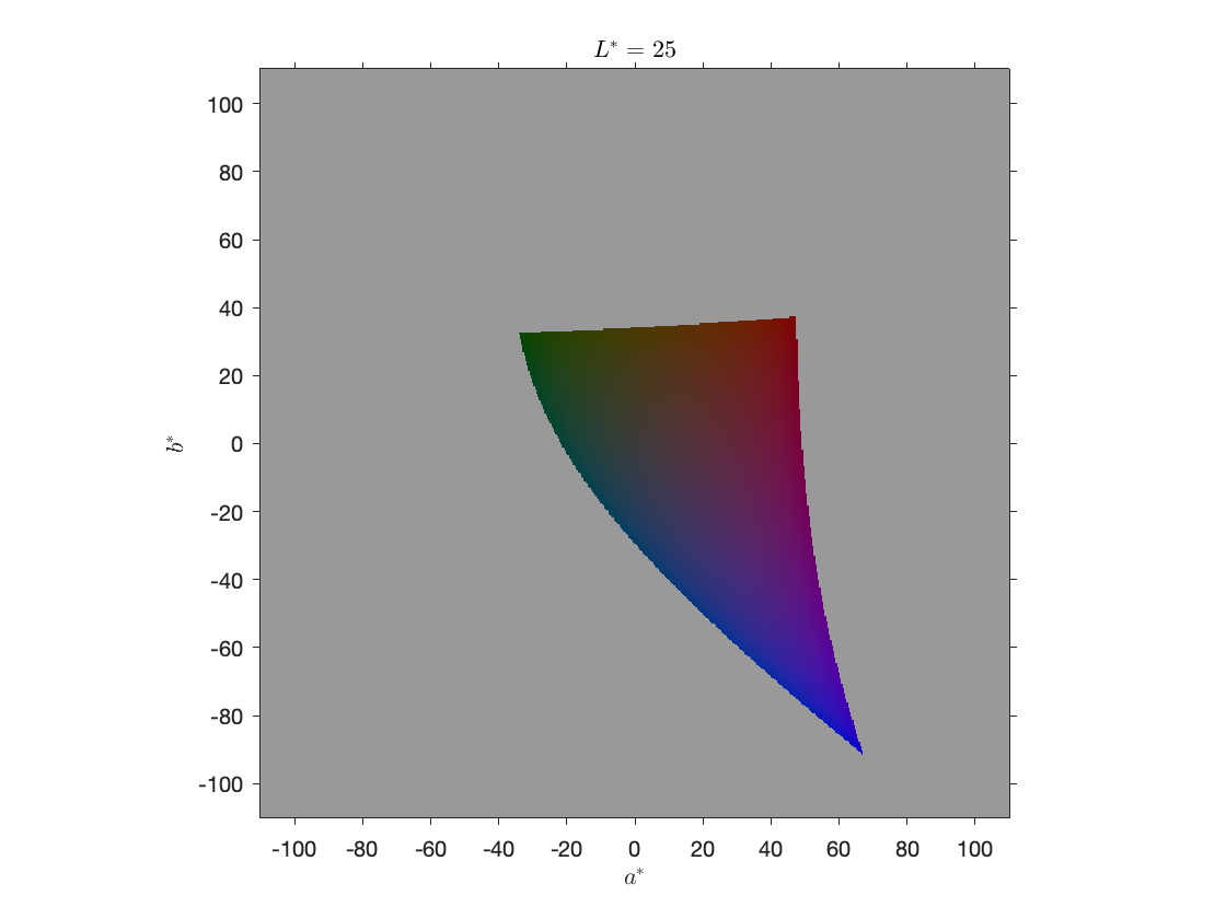
Although you can make out some relatively unsaturated green and red regions above, blue is the only fully saturated color.
What is the in-gamut$ (a^*,b^*) $region for every$ L^* $?
Now, I want to make multidimensional cubes of
$ L^* $
,
$ a^* $
, and
$ b^* $
values over their entire ranges and calculate the in-gamut colors all at once.
Find
$ L^* $
,
$ a^* $
,
$ b^* $
values filling a three-dimensional region. Convert the triples to sRGB.
L = 0:100;
[LL,bb,aa] = ndgrid(L,b,a);
rgb = lab2rgb([LL(:) aa(:) bb(:)]);
Reshape so that the color component is in the 4th dimension. Make a three-dimensional out-of-gamut mask. Replace out-of-gamut values with gray.
rgb = reshape(rgb,[size(LL) 3]);
mask = any((rgb > 1) | (rgb < 0),4);
rgb(repmat(mask,1,1,3)) = 0.6;
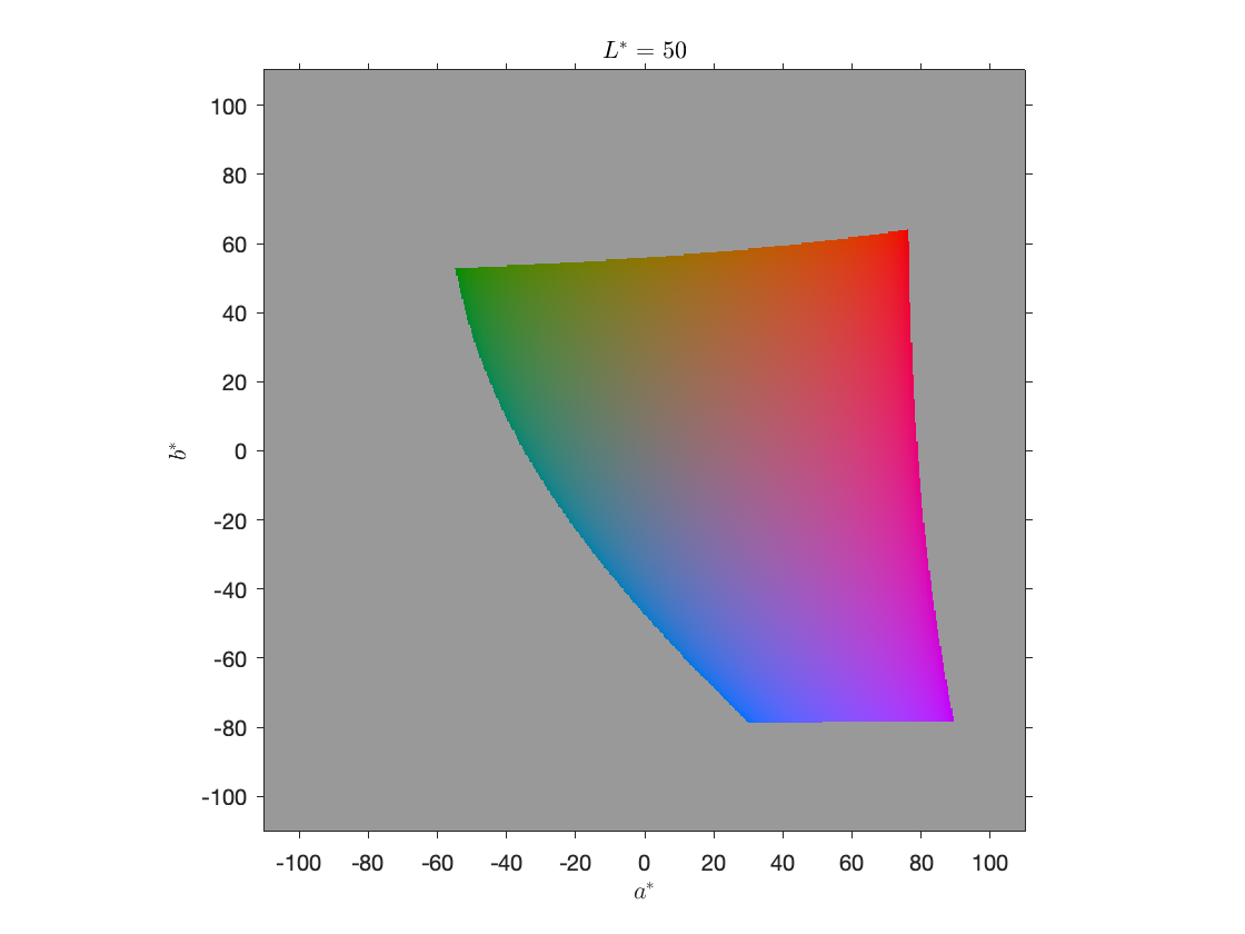
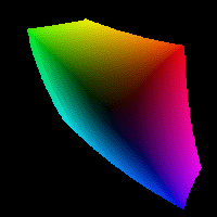
Display the set of colors for
$ L^*=50 $
(corresponding to the index 51 in the first dimension). After indexing with 51 in the first dimension, use
squeeze
to eliminate that dimension before displaying as an image.
rgb_50 = squeeze(rgb(51,:,:,:));
imshow(rgb_50,'XData',b,'YData',a)
axisxy
axison
xlabel('$a^*$','Interpreter','latex')
ylabel('$b^*$','Interpreter','latex')
title('$L^*=50$','Interpreter','latex')
Here's an animation, creating using
imwrite
, showing the in-gamut colors for the values of
$ L^* $
ranging from 0 to 100.

What is the in-gamut$ L^* $range everywhere in the$ (a^*,b^*) $plane?
These experiments caused me to wonder how to visualize the range of colors more broadly, while keeping the visualization in the
$ (a^*,b^*) $
plane. Here's a relevant question: given particular
$ a^* $
and
$ b^* $
values, what is the lowest
$ L^* $
value that is in gamut? What is the highest value? Further, can we tell if
no
$ L^* $
values are in gamut for a particular
$ a^* $
and
$ b^* $
?
I worked this out based on the multidimensional arrays computed above.
Find the minimum in-gamut values in the
LL
array along the first dimension, taking advantage of the fact that the
min
function ignores
NaN
values by default. Use the
squeeze
function to eliminate the first dimension, which has a size of 1 following the
min
operation.
LL_min = LL;
LL_min(mask) = NaN;
LL_min = squeeze(min(LL_min,[],1));
Following a similar procedure, find the maximum in-gamut values in the
LL
array along the first dimension.
LL_max = LL;
LL_max(mask) = NaN;
LL_max = squeeze(max(LL_max,[],1));
Here are the darkest and brightest in-gamut
$ L^* $
values on the
$ (a^*,b^*) $
plane, displayed with a grayscale colormap, along with the associated colors.
tiledlayout(2,2)
nexttile(1)
imshow(LL_min,[],'XData',a,'YData',b)
axisxy
axison
title('Minimum in-gamut $L^*$','Interpreter','latex')
xlabel('$a^*$','Interpreter','latex')
ylabel('$b^*$','Interpreter','latex')
nexttile(2)
imshow(LL_max,[],'XData',a,'YData',b)
axisxy
axison
title('Maximum in-gamut $L^*$','Interpreter','latex')
xlabel('$a^*$','Interpreter','latex')
ylabel('$b^*$','Interpreter','latex')
nexttile(3)
[aa,bb] = meshgrid(a,b);
rgb_min = lab2rgb(cat(3,LL_min,aa,bb));
imshow(rgb_min,'XData',a,'YData',b)
axisxy
axison
xlabel('$a^*$','Interpreter','latex')
ylabel('$b^*$','Interpreter','latex')
nexttile(4)
rgb_max = lab2rgb(cat(3,LL_max,aa,bb));
imshow(rgb_max,'XData',a,'YData',b)
axisxy
axison
xlabel('$a^*$','Interpreter','latex')
ylabel('$b^*$','Interpreter','latex')

Finally, I want to make an animation showing how the colors in the above plot change as they go from the darkest available color to the lightest, starting with another four-dimensional cube of RGB images:
N = 96;
[bb2,aa2] = ndgrid(b,a);
rgb_scan = zeros([size(bb2) 3 (N+1)]);
LL_diff = LL_max - LL_min;
fork = 0:N
L_k = LL_min + (LL_diff * (k/N));
rgb_scan(:,:,:,k+1) = lab2rgb(cat(3,L_k,aa2,bb2));
end
Here's the resulting animation, also created using
imwrite
. (Note that quality of the animation suffers because of the GIF limitation of no more than 256 distinct colors in each frame.)


评论
要发表评论,请点击此处登录到您的 MathWorks 帐户或创建一个新帐户。