It's March, and you know what that means --- that's right, the "a" release is here!On most work days, I use several different MATLAB versions, mostly development builds, on 2-3 different computers. But every March and September, I look forward to visiting mathworks.com/download to grab and install the latest real thing.Image Processing Toolbox (release notes) has several new deep learning examples, including this one about anomaly detection example using pretrained ResNet-18.Computer Vision Toolbox (release notes) added quite a lot in this release. For example, check out the ground truth

...read more >>

I have written here, as well as in Digital Image Processing Using MATLAB, about using image processing operations to implement Conway's Game of Life. MATLAB creator Cleve Moler has written about the Game of Life several times (03-Sep-2012, 10-Sep-2012, 17-Sep-2012, and 08-Nov-2018) on Cleve's Corner. Recently, I saw a particularly concise implementation of the game. My MathWorks

...read more >>

I was looking today at an old post, "A Lab-based uniform color scale" (09-May-2006). I wanted to provide an update to illustrate that it is easier to convert from Lab to RGB colors now than it was then. When I reread the original post, though, I realized that I was naive back then about the possibility that constructing a colormap using a path in Lab space could result in out-of-gamut colors when converting to sRGB.After thinking it over, I think I'd like to do two (or maybe three) follow-up posts. The first follow-up post, today, will focus on some ways to visualize where a curve in Lab space goes out-of-gamut for sRGB. Next, I'll explore ways to modify the technique I demonstrated previously in order to avoid out-of-gamut colors.Here is the colormap I showed in the 09-May-2006 post:radius = 50;theta = linspace(0, pi/2, 256).';a = radius * cos(theta);b = radius * sin(theta);L = linspace(0,

...read more >>

Today, I'm continuing my recent theme of thinking about peak-finding in images. When I wrote the first one (19-Aug-2021), I didn't realize it was going to turn into a series. This might be the last one—but no promises!My previous post (17-Sep-2021) was based on 1-D examples. Today's post focuses on an image example (in 2-D), and it connects to using regionprops to compute gray-weighted centroids of peaks. I'll also throw in some 3-D surface visualization, just for fun. Here is today's image:url = "https://blogs.mathworks.com/steve/files/snowflakes2.png";A = imread(url);imshow(A)I'd like to see if we can focus algorithmically on these white blobby things (that's a technical term that I learned in engineering school). First, let's try computing the

...read more >>

Last time, I introduced the idea of a regional maximum. Today, I want to add a concept that makes the regional maximum more useful: suppressing very small local maxima, possibly present only because of noise, that are are unimportant, before identifying the regional maxima. This "small peak suppression" can be accomplished using something called the h-maxima transform. The functions of interest today: imregionalmax, imhmax, imextendedmax, imregionalmin, imhmin, and imextendedmin. Let's get there by starting once again with the definition of regional maximum: a connected component of pixels with a constant value h, where every pixel that is neighbor to that connected component has a value that is lower than h. I'd like to elaborate on that using a one-dimensional example.y = peaksAndPlateaus;x = 1:length(y);plot(x,y)axis([-5 105 0 120])grid onI'll use dilation and

...read more >>

A recent algorithm discussion on the Image Processing Toolbox development team reminded me of something I originally wanted to do a long time ago: explain imregionalmax and some related operations. (I guess I got sidetracked.)For this explanation, I'll use the following sample image:P = sampleImage;imshow(P)Note that this image has a number of constant-valued rings. One might call these regions "plateaus." Here is a cross-section of the pixel values:p256 = P(256,:);plot(p256)axis([1 500 0 300])text(250,255,"plateau",HorizontalAlignment = "center", ... VerticalAlignment = "bottom")text(345,204,"plateau",HorizontalAlignment = "center", ... VerticalAlignment = "bottom")text(415,153,"plateau",HorizontalAlignment = "center", ... VerticalAlignment = "bottom")text(471,102,"plateau",HorizontalAlignment = "center", ... VerticalAlignment = "bottom")Local maximaIn image processing, the usual definition of a local maximum is that a pixel is considered to be a local maximum if and only

...read more >>

The functions meshgrid and repmat have a long and rich history in MATLAB. Today, I'll try to convince you to use them less.meshgridThe function meshgrid is typically used to take a vector of x-coordinates and a vector of y-coordinates and turn them into two matrices, X and Y, that can be used to compute a function of two variables. Here is a small example.x = [0 1 2];y = [0 10 20 30];[X,Y] = meshgrid(x,y)X = 4×3 0 1 2 0 1 2 0 1 2 0 1 2 Y = 4×3 0 0 0 10 10 10 20 20 20 30 30 30 Here is another example that illustrates how meshgrid is typically used. The example, taken from the 2nd edition (2009) of Digital Image Processing Using MATLAB, constructs a surface plot of the function $ f(x,y) = xe^{-(x^2 + y^2)} $.x = -2:0.1:2;y = -2:0.1:2;[X,Y] = meshgrid(x,y);Z = X.*exp(-(X.^2 + Y.^2));surf(Z)The variables x and y are vectors, and the variables X and Y are matrices:whos x y X Y Name

...read more >>

Today, I want to convince you to use imbinarize instead of im2bw.Background: I recently saw some data suggesting that many Image Processing Toolbox users are still using im2bw, an old function that dates back to the original toolbox release in 1993. We recommend using the newer function, imbinarize, because it saves a step in the most common scenario, and because it offers additional flexibility if you need it.I'll explain by updating an old blog post topic called "Tracing George," in which I try to extract the curve shown in the following image:url = 'https://blogs.mathworks.com/images/steve/36/george.jpg';I = imread(url);imshow(I)I call this "George." I created George originally for some examples and diagrams in the book Digital Image Processing Using MATLAB. I found at some point that I needed to reproduce the outline curve, but I

...read more >>

Some of us at MathWorks like to share our "NaN sightings." Here is an example to show what I mean. This is a screenshot of the tuner/metronome app that I use when practicing music. One day, I was a bit startled when the app suddenly decided that my metronome tempo was -NaN. (Am I playing too fast? No. Am I playing too slow? No. Am I playing at just the right speed? Also no.)

Here's another example spotted by a fellow MathWorker. In a town near my home, you can apparently buy a lawn tractor that has been driven NaN miles.

And a third MathWorker was helping a family member file their taxes and received this surprising summary of the results.

If you spot some amusing NaNs in the wild, let us

...read more >>

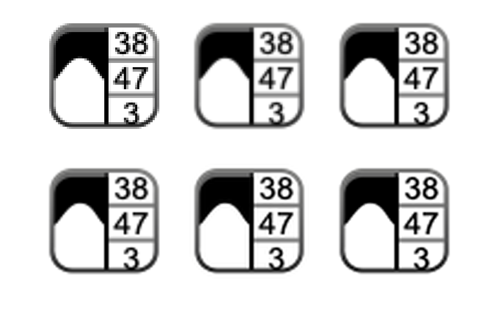
Recently, I was talking with MathWorks writer Jessica Bernier about the reference page for the imresize function. Jessica pointed out that we don't have an example that shows how to use your own interpolation kernel. In today's post, I'll compare the supported interpolation kernels on a sample image, and then I'll show you how to use your own kernel.The different methods supported by imresize, including 'bilinear', 'bicubic', 'lanczos2', and 'lanczos3', correspond to using different interpolation kernels, also known as interpolants. The bilinear method uses a triangular interpolation kernel, which is defined as:f(x)={1-|x||x|≤10otherwisefplot(@triangle,[-3.5 3.5])(The function triangle, as well as the other interpolation kernel functions used in this post, are at the end.)The bicubic method uses this piecewise cubic interpolation

...read more >>