Load Pretrained Network

Load a pretrained GoogLeNet network.

net = googlenet;

Visualize Early Convolutional Layers

There are multiple convolutional layers in the GoogLeNet network. The convolutional layers towards the beginning of the network have a small receptive field size and learn small, low-level features. The layers towards the end of the network have larger receptive field sizes and learn larger features.

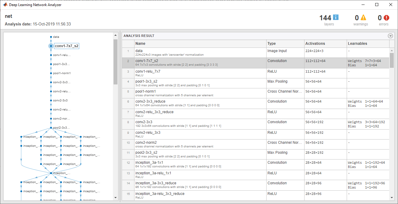
UsinganalyzeNetwork, view the network architecture and locate the convolutional layers.

analyzeNetwork(net)

Features on Convolutional Layer 1

Setlayerto be the first convolutional layer. This layer is the second layer in the network and is named'conv1-7x7_s2'.

layer = 2; name = net.Layers(layer).Name

name = 'conv1-7x7_s2'

Visualize the first 36 features learned by this layer usingdeepDreamImageby settingchannelsto be the vector of indices1:36. Set'PyramidLevels'1,这样的图像缩放。到display the images together, you can useimtile.

deepDreamImage使用一个兼容的GPU,默认情况下,如果可用。Otherwise it uses the CPU. A CUDA® enabled NVIDIA® GPU with compute capability 3.0 or higher is required for running on a GPU.

channels = 1:36; I = deepDreamImage(net,name,channels,...'PyramidLevels',1);

|==============================================| | Iteration | Activation | Pyramid Level | | | Strength | | |==============================================| | 1 | 0.26 | 1 | | 2 | 6.99 | 1 | | 3 | 14.24 | 1 | | 4 | 21.49 | 1 | | 5 | 28.74 | 1 | | 6 | 35.99 | 1 | | 7 | 43.24 | 1 | | 8 | 50.50 | 1 | | 9 | 57.75 | 1 | | 10 | 65.00 | 1 | |==============================================|

figure I = imtile(I,'ThumbnailSize',[64 64]); imshow(I) title(['Layer ',name,' Features'],'Interpreter','none')

These images mostly contain edges and colors, which indicates that the filters at layer'conv1-7x7_s2'are edge detectors and color filters.

Features on Convolutional Layer 2

The second convolutional layer is named'conv2-3x3_reduce', which corresponds to layer 6. Visualize the first 36 features learned by this layer by settingchannelsto be the vector of indices1:36.

To suppress detailed output on the optimization process, set'Verbose'to'false'in the call todeepDreamImage.

layer = 6; name = net.Layers(layer).Name

name = 'conv2-3x3_reduce'

channels = 1:36; I = deepDreamImage(net,name,channels,...'Verbose',false,...'PyramidLevels',1); figure I = imtile(I,'ThumbnailSize',[64 64]); imshow(I) name = net.Layers(layer).Name; title(['Layer ',name,' Features'],'Interpreter','none')

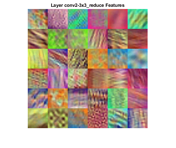
Filters for this layer detect more complex patterns than the first convolutional layer.

Visualize Deeper Convolutional Layers

The deeper layers learn high-level combinations of features learned by the earlier layers.

Increasing the number of pyramid levels and iterations per pyramid level can produce more detailed images at the expense of additional computation. You can increase the number of iterations using the'NumIterations'option and increase the number of pyramid levels using the 'PyramidLevels' option.

layer = 97; name = net.Layers(layer).Name

name = 'inception_4e-1x1'

channels = 1:6; I = deepDreamImage(net,name,channels,...'Verbose',false,..."NumIterations",20,...'PyramidLevels',2); figure I = imtile(I,'ThumbnailSize',[250 250]); imshow(I) name = net.Layers(layer).Name; title(['Layer ',name,' Features'],'Interpreter','none')

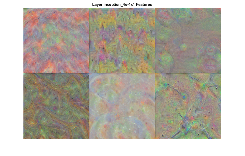
Notice that the layers which are deeper into the network yield more detailed filters which have learned complex patterns and textures.

Visualize Fully Connected Layer

To produce images that resemble each class the most closely, select the fully connected layer, and setchannelsto be the indices of the classes.

Select the fully connected layer (layer 142).

layer = 142; name = net.Layers(layer).Name

name = 'loss3-classifier'

Select the classes you want to visualize by settingchannelsto be the indices of those class names.

channels = [114 293 341 484 563 950];

The classes are stored in theClassesproperty of the output layer (the last layer). You can view the names of the selected classes by selecting the entries inchannels.

net.Layers(end).Classes(channels)

ans =6×1 categoricalsnail tiger zebra castle fountain strawberry

Generate detailed images that strongly activate these classes. Set'NumIterations'to 100 in the call todeepDreamImageto produce more detailed images. The images generated from the fully connected layer correspond to the image classes.

I = deepDreamImage(net,name,channels,...'Verbose',false,...'NumIterations', 100,...'PyramidLevels',2); figure I = imtile(I,'ThumbnailSize',[250 250]); imshow(I) name = net.Layers(layer).Name; title(['Layer ',name,' Features'])

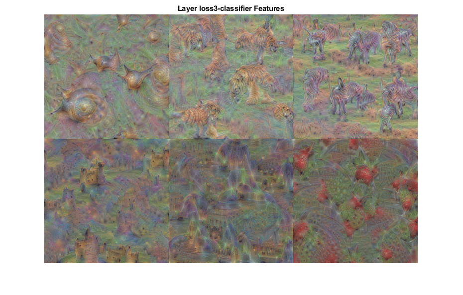
The images generated strongly activate the selected classes. The image generated for the ‘zebra’ class contain distinct zebra stripes, whilst the image generated for the ‘castle’ class contains turrets and windows.