在此视频中,您将学习如何使用MATLAB中的部分微分方程工具箱进行有限元方法进行结构分析。部分微分方程可以代表从简单的悬臂变形,主板中的散热到喷射涡轮机叶片的热机械应力的物理问题。在该视频中,我们将专注于对来自周围气体的压力进行压力的涡轮叶片进行结构分析。但首先是什么是喷气式涡轮机叶片?飞机上的喷气发动机负责产生使飞机飞行的推力。在喷射发动机内,涡轮机,叶片的径向阵列从燃烧室中产生的高温和高压气体提取能量,并将其转化为旋转运动以产生推力。涡轮叶片在极高的温度和压力下被气体包围。刀片材料均显着膨胀和变形,在接头中产生机械应力,并且几毫米的显着变形。为避免刀片尖端和涡轮机壳之间的机械故障和摩擦,刀片设计必须考虑遇险和变形。让我们现在看看我们如何在Matlab中做到这一点。 We start by creating a PDE model object that determines the type of analysis we're performing using the create PDE command. To perform a structural analysis, we indicate that as the first argument. We then specify the model to be a static solid model. The PDE Toolbox supports various other types of analysis, such as transient, mortal, etc. We will be using the model object later on to set up the analysis. In a typical finite element analysis workflow, we go through four steps. Import or create geometry. Preprocess to geometry. Solve the problem. Post process the results. After defining the analysis type, we begin with the first step of the analysis. Import the geometry of the blade model from an STL file. STL is a common file format and supported by most CAD software. Alternatively, you could also create simple geometry is natively. The importGeometry command creates a geometry container from the specified STL geometry file and includes the geometry in the model container. We can then plot the geometry of the blade using the pdegplot command with face labels and the transparency of the faces. We can then view the blade geometry from multiple angles. Next, we will discretize the geometry into finite elements. The generateMesh command is used to generate a mesh for the geometry of the blade. The mesh is a collection of elements with vertices, edges and faces that defines the geometry. We set the maximum edge length of the elements to be 0.01 using the HMax parameter. The mesh can be visualized using pdeplot3D. We can then view the mesh from multiple angles. We then define the physics of the problem. So far, the model does not contain any information of the material or structural properties of the material. In this example, the blade is made of a nickel-based alloy called Mnemonic 90. Two properties of this alloy are of importance for the analysis, Young's modulus, denoted by eta, measure of the stiffness of the material and poisons ratio denoted by nu, a measure of the deformation of the material. We then use the structural properties command to set the material properties of smodel. All the faces of the blade are free to deform except for face 3. Face three is fixed to the radial axis of the turbine. This restriction can be imposed as a boundary condition of the model using the structuralBC function. We first specify the face which the constraint is being applied to, which is 3 in this case and then specify the constraint type fixed. The pressure of the surrounding gases deforms the blade from either side. The pressure load on the pressure side of the blade is 5e5 pascal and deforms the blade towards the suction side. Whereas the pressure load on the suction side of the blade is 4.5e5 pascal and informs the blade towards the pressure side. We can apply this pressure loads on the model using the structural boundary load function. First, we specify the pressure on the pressure side of the blade. That is, the pressure on face 11 as 5e5 pascal. And then a slightly lower pressure of 4.5e5 pascal on the suction side. Finally, we solve the problem using the solve command. We can then post process the results and visualize it. The pdeplot3D command can then be used to visualize the stress and deformed shape of the model. Here we are looking at the von-misses stress of the deformed shape. The deformation scale factor is set 200 to make the deformation easier to visualize. The colors correspond to the stress levels of the blade and various points. The maximum stress is found at the tip of the blade around 100 megapascal, which is still significantly below the elastic limit of the alloy, indicating that the blade will not permanently deform under the pressure load. Once the model is built, you may want to explore the design space using design of experiment techniques or by simply doing parameter sweeps. Please check out the statistics and machine learning toolbox for more information. You may also want to optimize your design for specific conditions or find the best material to be used for specific applications. In the video we just covered, you learn how to perform structural analysis using finite element method with partial differential equation toolbox in MATLAB. To learn more about using the PDE toolbox, please refer to the PDE toolbox home page and the examples on the documentation page. In an upcoming video, will analyze heat transfer on the same blade. Don't forget to check out the links in the video description. Thank you for watching.