Hello. In this video, we will show how to design and simulate a digital control algorithm for power factor correction.
在这里,我们使用SIMSCAPE电气和Simulink的块对典型的活动功率因数校正设置进行了建模。金宝app让我们看一下模型的不同元素。我们有一个连接到二极管桥梁整流器的120V RMS的交流源。该整流器连接到数字控制的升压转换器和额定400V的电阻载荷。
我们已经模拟了该服务l control algorithm in this subsystem named Controls. We can see the algorithm is a cascaded control loop architecture. The outer loop controls the load voltage and the inner loop controls the inductor current.
我们的控制算法计算一个PWM信号,该信号驱动增压转换器的MOSFET。在此视频中,我们不会讨论被动组件的大小。我们将在模型中与已经有电感和电容的参数值一起工作,但是重要的是要注意,我们可以轻松更改这些值,运行仿真并观察变化。因此,我们可以使用此仿真模型为被动组件选择最佳参数值,但是我们的重点是数字控制算法。
In this model, the PI gains for the controllers were set as initial guesses. These gain values do not provide the best power factor correction. We can see that by running the model. In this plot we see the line voltage in yellow and the line current in blue. The current waveform shows the presence of harmonics, which results in a poor power factor. We will therefore need to retune the controllers for a better power factor correction.
Our workflow will be the following: We will first tune the inner loop to obtain the optimal PID gains for the current loop. With the inner loop tuned, we will tune the outer voltage loop to compute gains for voltage loop PI controller.
要进行调整,我们需要获得线性植物动力学模型。对于内部循环,我们需要从PWM占空比到电感电流获得动力学。我们将使用Simulink控制设计中的线性分析工具来做到这一点。金宝app使用此工具,我们可以通过进行AC扫描来估计模型的频率响应。我们需要围绕适当的工作点或偏置点进行此操作。要进行交流扫描,我们必须用直流源代替交流电压源。
This model has been set up to operate at its DC operating point with a DC voltage source of 120V and a steady state duty cycle of 0.72 [AT1] to maintain a constant DC output of 400V.
We can specify that we are interested in the dynamics from the PWM duty cycle to the inductor current by marking those signals as input and output linearization points respectively. The simulation reaches steady state at about ~0.15 seconds, so we will the start frequency response estimation at that time when the steady state has been reached. Next, we specify that we will inject the fixed step sine stream input with a sample time of 0.2 microseconds to the model. We set the frequency sweep range from 10Hz to 15kHz and the amplitude of the signal to 0.036 to ensure sufficient excitation within the operating range. We choose this signal amplitude to be small enough to not take us away from our operating point.
We then start the frequency response estimation. The model is simulated and the plant frequency response is computed. We will export it to the MATLAB workspace to use for the PI controller tuning.
In this next step we set up the current PI controller in the controls subsystem with the reference and the measured inductor current to operate in closed loop.
Next, we tune the gains of PI controller block by pressing the tune button in the block dialog. This launches the PID Tuner that tries to automatically linearize the plant. Because in this model we have discontinuities such as MOSFETs and PWM switching, the model cannot be linearized analytically. However, this is okay because this is exactly why we ran the frequency response estimation before. We can now simply point the PID Tuner to the estimated frequency response.
The PID Tuner uses this frequency response to compute PI gains to provide fast and stable closed-loop operation of the system. We can use the sliders to adjust the bandwidth and the phase margin. We will tune for the bandwidth of around 3.760 kHz and phase margin of 60 degrees to maintain a robust current reference tracking.
We can now take the computed PI gains and update them in the PI block of our model.
通过调整内部电流循环,我们将重复该过程以调整外电压循环。在控件子系统中,此处1的常数块表示电感器电流请求。在我们的最终模型中,该信号将由外电压循环计算。因此,为了调整外循环,我们的输入线性化点是该信号,输出线性化点是输出电压信号。
The simulation reaches steady state at around 0.4 seconds, so we will tell the Linear Analysis tool to start the frequency response estimation at around that time. We set the fixed step sine stream signal sample time to 0.2 microseconds with an AC frequency sweep range from 10Hz to 5kHz. The amplitude of the perturbation is set to be 0.1 to ensure sufficient excitation. We can now run the tool and compute the frequency response for tuning the outer loop.
Next, just like we did for the inner loop, we will set up the outer loop Controls subsystem with the Voltage PI controller, and start the tuning by launching the PID Tuner. Again, similar to how we did it for the inner loop, we import the previously estimated frequency response to compute the PI gains. The voltage loop is slower than the inner current loop, so we set the bandwidth to be around 55 Hz and keep phase margin at 60 degrees. With this chosen bandwidth, the controller will follow the reference voltage while rejecting the 120Hz oscillations of the rectified AC source.
We then update the voltage PI Controller with the computed gains. To verify the performance in the nonlinear model, let’s run a step change in the reference voltage. The simulation results show a robust controller performance.
现在,让我们将电压源切回原始的交流电网并运行仿真。
我们可以看到电感电流和输出电压轮廓显示出良好的参考跟踪。从AC网格绘制的线电流类似于完美的正弦曲线,并且比控制器调整之前的当前轮廓要好得多。我们看到谐波的减少,从而提供了更好的功率因素。
To summarize, in this video we showed how to simulate, design, and tune a digital control algorithm for power factor correction in Simulink. With the design complete, a good next step would be to generate code from the Controls subsystem to deploy on an embedded controller to be tested with a physical plant. This concludes the video.