Simulate the Motion of the Periodic Swing of a Pendulum

Open Live Script

This example shows how to simulate the motion of a simple pendulum using Symbolic Math Toolbox™. Derive the equation of motion of the pendulum, then solve the equation analytically for small angles and numerically for any angle.

Step 1: Derive the Equation of Motion

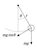
The pendulum is a simple mechanical system that follows a differential equation. The pendulum is initially at rest in a vertical position. When the pendulum is displaced by an angle $θ$ and released, the force of gravity pulls it back towards its resting position. Its momentum causes it to overshoot and come to an angle $- θ$ (if there are no frictional forces), and so on. The restoring force along the motion of the pendulum due to gravity is $- m g \sin θ$ 。因此,根据牛顿第二定律,质量times the acceleration must equal $- m g \sin θ$ 。

symsmagtheta(t)eqn = m*a == -m*g*sin(theta)

eqn(t) =
                   $a m = - g m \sin (θ (t))$

For a pendulum with length $r$ , the acceleration of the pendulum bob is equal to the angular acceleration times $r$ 。

$a = r \frac{d^{2} θ}{d t^{2}}$ 。

Substitute for $a$ by usingsubs。

symsreqn = subs(eqn,a,r*diff(theta,2))

eqn(t) =
                  
                    $m r \frac{\partial^{2}}{\partial t^{2}} θ (t) = - g m \sin (θ (t))$

Isolate the angular acceleration ineqnby usingisolate。

eqn = isolate(eqn,diff(theta,2))

eqn =
                  
                    $\frac{\partial^{2}}{\partial t^{2}} θ (t) = - \frac{g \sin (θ (t))}{r}$

Collect the constants $g$ and $r$ into a single parameter, which is also known as thenatural frequency。

$ω_{0} = \sqrt{\frac{g}{r}}$ 。

symsomega_0eqn = subs(eqn,g/r,omega_0^2)

eqn =
                  
                    $\frac{\partial^{2}}{\partial t^{2}} θ (t) = - {ω_{0}}^{2} \sin (θ (t))$

Step 2: Linearize the Equation of Motion

The equation of motion is nonlinear, so it is difficult to solve analytically. Assume the angles are small and linearize the equation by using the Taylor expansion of $\sin θ$ 。

symsxapprox = taylor(sin(x),x,'Order',2); approx = subs(approx,x,theta(t))

approx =
                   $θ (t)$

The equation of motion becomes a linear equation.

eqnLinear = subs(eqn,sin(theta(t)),approx)

eqnLinear =
                  
                    $\frac{\partial^{2}}{\partial t^{2}} θ (t) = - {ω_{0}}^{2} θ (t)$

Step 3: Solve Equation of Motion Analytically

Solve the equationeqnLinearby usingdsolve。Specify initial conditions as the second argument. Simplify the solution by assuming $ω_{0}$ is real usingassume。

symstheta_0theta_t0theta_t = diff(theta); cond = [theta(0) == theta_0, theta_t(0) == theta_t0]; assume(omega_0,'real') thetaSol(t) = dsolve(eqnLinear,cond)

thetaSol(t) =
                  
                    $θ_{0} \cos (ω_{0} t) + \frac{θ_{t0} \sin (ω_{0} t)}{ω_{0}}$

Step 4: Physical Significance of $ω_{0}$

The term $ω_{0} t$ is called thephase。The cosine and sine functions repeat every $2 π$ 。The time needed to change $ω_{0} t$ by $2 π$ is called the time period.

$T = \frac{2 π}{ω_{0}} = 2 π \sqrt{\frac{r}{g}}$ 。

The time period $T$ is proportional to the square root of the length of the pendulum and it does not depend on the mass. For linear equation of motion, the time period does not depend on the initial conditions.

Step 5: Plot Pendulum Motion

Plot the motion of the pendulum for small-angle approximation.

Define the physical parameters:

Gravitational acceleration $g = 9 。 81 {m/s}^{2}$
Length of pendulum $r = 1 m$

gValue = 9.81; rValue = 1; omega_0Value = sqrt(gValue/rValue); T = 2*pi/omega_0Value;

设置初始条件。

theta_0Value = 0.1*pi;% Solution only valid for small angles.theta_t0Value = 0;% Initially at rest.

Substitute the physical parameters and initial conditions into the general solution.

var = [omega_0 theta_0 theta_t0];值=(ω_0Value theta_0Value theta_t0Value]; thetaSolPlot = subs(thetaSol,vars,values);

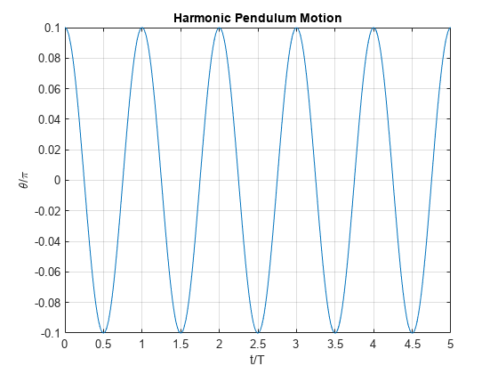
Plot the harmonic pendulum motion.

fplot(thetaSolPlot(t*T)/pi, [0 5]); gridon; title('Harmonic Pendulum Motion'); xlabel('t/T'); ylabel('\theta/\pi');

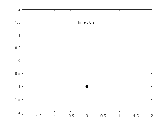
Figure contains an axes object. The axes object with title Harmonic Pendulum Motion, xlabel t/T, ylabel theta / pi contains an object of type functionline.

After finding the solution for $θ (t)$ , visualize the motion of the pendulum.

x_pos = sin(thetaSolPlot); y_pos = -cos(thetaSolPlot); fanimator(@fplot,x_pos,y_pos,'ko','MarkerFaceColor','k','AnimationRange',[0 5*T]); holdon; fanimator(@(t) plot([0 x_pos(t)],[0 y_pos(t)],'k-'),'AnimationRange',[0 5*T]); fanimator(@(t) text(-0.3,0.3,"Timer: "+num2str(t,2)+" s"),'AnimationRange',[0 5*T]);

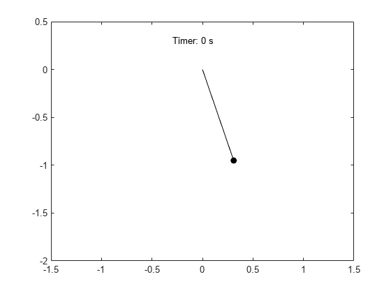
Figure contains an axes object. The axes object contains 3 objects of type parameterizedfunctionline, line, text.

Enter the commandplayAnimationto play the animation of the pendulum motion.

Step 6: Determine Nonlinear Pendulum Motion Using Constant Energy Paths

To understand the nonlinear motion of the pendulum, visualize the pendulum path by using the equation for total energy. The total energy is conserved.

$E = \frac{1}{2} m r^{2} {(\frac{d θ}{dt})}^{2} + m g r (1 - \cos θ)$

Use the trigonometric identity $1 - \cos θ = 2 \sin^{2} (θ / 2)$ and the relation $ω_{0} = \sqrt{g / r}$ to rewrite the scaled energy.

$\frac{E}{m r^{2}} = \frac{1}{2} [{(\frac{d θ}{dt})}^{2} + {(2 ω_{0} \sin \frac{θ}{2})}^{2}]$

Since energy is conserved, the motion of the pendulum can be described by constant energy paths in the phase space. The phase space is an abstract space with the coordinates $θ$ and $d θ / d t$ 。Visualize these paths usingfcontour。

symsthetatheta_tomega_0E(theta, theta_t, omega_0) = (1/2)*(theta_t^2+(2*omega_0*sin(theta/2))^2); Eplot(theta, theta_t) = subs(E,omega_0,omega_0Value); figure; fc = fcontour(Eplot(pi*theta, 2*omega_0Value*theta_t), 2*[-1 1 -1 1],。..'LineWidth', 2,'LevelList', 0:5:50,'MeshDensity', 1+2^8); gridon; title('Constant Energy Contours in Phase Space ( \theta vs. \theta_t )'); xlabel('\theta/\pi'); ylabel('\theta_t/2\omega_0');

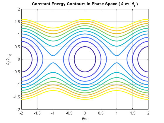
Figure contains an axes object. The axes object with title Constant Energy Contours in Phase Space ( blank theta blank v s . blank theta indexOf t baseline blank ), xlabel theta / pi, ylabel theta indexOf t baseline / 2 omega indexOf 0 baseline contains an object of type functioncontour.

The constant energy contours are symmetric about the $θ$ axis and $d θ / d t$ axis, and are periodic along the $θ$ axis. The figure shows two regions of distinct behavior.

The lower energies of the contour plot close upon themselves. The pendulum swings back and forth between two maximum angles and velocities. The kinetic energy of the pendulum is not enough to overcome gravitational energy and enable the pendulum to make a full loop.

The higher energies of the contour plot do not close upon themselves. The pendulum always moves in one angular direction. The kinetic energy of the pendulum is enough to overcome gravitational energy and enable the pendulum to make a full loop.

Step 7: Solve Nonlinear Equations of Motion

The nonlinear equations of motion are second-order differential equations. Numerically solve these equations by using theode45solver. Becauseode45accepts only first-order systems, reduce the system to a first-order system. Then, generate function handles that are the input toode45。

Rewrite the second-order ODE as a system of first-order ODEs.

symstheta(t)theta_t(t)omega_0eqs = [diff(theta) == theta_t; diff(theta_t) == -omega_0^2*sin(theta)]

eqs(t) =
                  
                    $(\begin{array}{c} \frac{\partial}{\partial t} θ (t) = θ_{t} (t) \\ \frac{\partial}{\partial t} θ_{t} (t) = - {ω_{0}}^{2} \sin (θ (t)) \end{array})$

eqs = subs(eqs,omega_0,omega_0Value); vars = [theta, theta_t];

Find the mass matrixMof the system and the right sides of the equationsF。

[M,F] = massMatrixForm(eqs,vars)

M =
                  
                    $(\begin{array}{c} 1 & 0 \\ 0 & 1 \end{array})$

F =
                  
                    $(\begin{array}{c} θ_{t} (t) \\ - \frac{981 \sin (θ (t))}{100} \end{array})$

MandFrefer to this form.

$M (t, x (t)) \frac{dx}{dt} = F (t, x (t)) 。$

To simplify further computations, rewrite the system in the form $d x / d t = f (t, x (t))$ 。

f = M\F

f =
                  
                    $(\begin{array}{c} θ_{t} (t) \\ - \frac{981 \sin (θ (t))}{100} \end{array})$

Convertfto a MATLAB function handle by usingodeFunction。The resulting function handle is the input to the MATLAB ODE solverode45。

f = odeFunction(f, vars)

f =function_handle with value:@ (t, in2) [in2(2:);罪(in2 (1,:)).*(-9.81e+2./1.0e+2)]

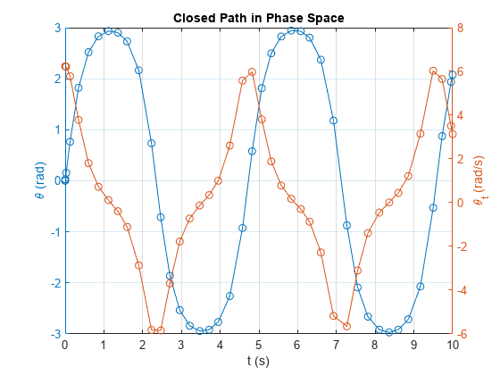
Step 8: Solve Equation of Motion for Closed Energy Contours

Solve the ODE for the closed energy contours by usingode45。

From the energy contour plot, closed contours satisfy the condition $θ_{0} = 0$ , $θ_{t 0} / 2 ω_{0} \leq 1$ 。Store the initial conditions of $θ$ and $d θ / d t$ in the variablex0。

x0 = [0; 1.99*omega_0Value];

Specify a time interval from 0 s to 10 s for finding the solution. This interval allows the pendulum to go through two full periods.

tInit = 0; tFinal = 10;

Solve the ODE.

sols = ode45(f,[tInit tFinal],x0)

sols =struct with fields:solver: 'ode45' extdata: [1x1 struct] x: [0 3.2241e-05 1.9344e-04 9.9946e-04 0.0050 0.0252 0.1259 0.3449 0.6020 0.8591 1.1161 1.3597 1.5996 1.8995 2.2274 2.4651 2.7028 2.9567 3.2138 3.4709 3.7150 3.9511 4.2483 4.5759 4.8239 5.0719 5.3182 5.5764 5.8346 6.0803 6.3072 6.5981 ... ] y: [2x45 double] stats: [1x1 struct] idata: [1x1 struct]

sols.y(1,:)represents the angular displacement $θ$ andsols.y(2,:)represents the angular velocity $d θ / d t$ 。

Plot the closed-path solution.

figure; yyaxisleft; plot(sols.x, sols.y(1,:),'-o'); ylabel('\theta (rad)'); yyaxisright; plot(sols.x, sols.y(2,:),'-o'); ylabel('\theta_t (rad/s)'); gridon; title('Closed Path in Phase Space'); xlabel('t (s)');

Figure contains an axes object. The axes object with title Closed Path in Phase Space, xlabel t (s), ylabel theta indexOf t baseline blank ( r a d / s ) contains 2 objects of type line.

Visualize the motion of the pendulum.

x_pos = @(t) sin(deval(sols,t,1)); y_pos = @(t) -cos(deval(sols,t,1)); figure; fanimator(@(t) plot(x_pos(t),y_pos(t),'ko','MarkerFaceColor','k')); holdon; fanimator(@(t) plot([0 x_pos(t)],[0 y_pos(t)],'k-')); fanimator(@(t) text(-0.3,1.5,"Timer: "+num2str(t,2)+" s"));

Figure contains an axes object. The axes object contains 3 objects of type line, text. One or more of the lines displays its values using only markers

Enter the commandplayAnimationto play the animation of the pendulum motion.

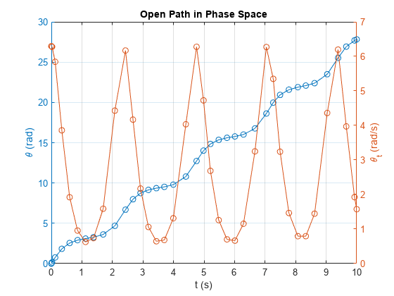
Step 9: Solutions on Open Energy Contours

Solve the ODE for the open energy contours by usingode45。From the energy contour plot, open contours satisfy the condition $θ_{0} = 0$ , $θ_{t 0} / 2 ω_{0} > 1$ 。

x0 = [0; 2.01*omega_0Value]; sols = ode45(f, [tInit, tFinal], x0);

Plot the solution for the open energy contour.

figure; yyaxisleft; plot(sols.x, sols.y(1,:),'-o'); ylabel('\theta (rad)'); yyaxisright; plot(sols.x, sols.y(2,:),'-o'); ylabel('\theta_t (rad/s)'); gridon; title('Open Path in Phase Space'); xlabel('t (s)');

Figure contains an axes object. The axes object with title Open Path in Phase Space, xlabel t (s), ylabel theta indexOf t baseline blank ( r a d / s ) contains 2 objects of type line.

Visualize the motion of the pendulum.

x_pos = @(t) sin(deval(sols,t,1)); y_pos = @(t) -cos(deval(sols,t,1)); figure; fanimator(@(t) plot(x_pos(t),y_pos(t),'ko','MarkerFaceColor','k')); holdon; fanimator(@(t) plot([0 x_pos(t)],[0 y_pos(t)],'k-')); fanimator(@(t) text(-0.3,1.5,"Timer: "+num2str(t,2)+" s"));

Figure contains an axes object. The axes object contains 3 objects of type line, text. One or more of the lines displays its values using only markers