我们将有一个分两部分的关于“波西米亚矩阵”的小型研讨会ICIAM20197月15日至19日，国际工业与应用数学大会在西班牙巴伦西亚召开。这是我演讲的提纲。

内容

为什么“波西米亚”

“波西米亚矩阵”这个五彩缤纷的名字是西安大略大学的Rob Corless和Steven Thornton提出的。引用网站。

当这个项目处于早期阶段时，我们的重点是有界高度的随机整数矩阵。我们最初使用短语“有界高度整数矩阵特征值”来指代我们的工作。这就产生了首字母缩略词BHIME，与“波西米亚”相差不远。

MATLAB图库

的画廊是一个有趣的矩阵集合，由Nick highham在MATLAB中维护。他们中的许多人都是波希米亚人，或者是波希米亚人的崇拜者。提供了该集合的目录

帮助gallery_

GALLERY海厄姆测试矩阵。着干活,out2,……= GALLERY(matname, param1, param2，…)接受matname(一个矩阵族的名称字符串)和该矩阵族的输入参数。请参阅下面的清单了解可用的矩阵族。大多数函数接受指定矩阵顺序的输入参数，除非另有说明，否则返回单个输出。有关其他信息，请键入“help private/matname”，其中matname是矩阵族的名称。二项式矩阵——对合矩阵的倍数。柯西柯西矩阵。Chebyshev谱微分矩阵。Chebyshev多项式的类Chebyshev矩阵。 chow Chow matrix -- a singular Toeplitz lower Hessenberg matrix. circul Circulant matrix. clement Clement matrix -- tridiagonal with zero diagonal entries. compar Comparison matrices. condex Counter-examples to matrix condition number estimators. cycol Matrix whose columns repeat cyclically. dorr Dorr matrix -- diagonally dominant, ill-conditioned, tridiagonal. (One or three output arguments, sparse) dramadah Matrix of ones and zeroes whose inverse has large integer entries. fiedler Fiedler matrix -- symmetric. forsythe Forsythe matrix -- a perturbed Jordan block. frank Frank matrix -- ill-conditioned eigenvalues. gcdmat GCD matrix. gearmat Gear matrix. grcar Grcar matrix -- a Toeplitz matrix with sensitive eigenvalues. hanowa Matrix whose eigenvalues lie on a vertical line in the complex plane. house Householder matrix. (Three output arguments) integerdata Array of arbitrary data from uniform distribution on specified range of integers invhess Inverse of an upper Hessenberg matrix. invol Involutory matrix. ipjfact Hankel matrix with factorial elements. (Two output arguments) jordbloc Jordan block matrix. kahan Kahan matrix -- upper trapezoidal. kms Kac-Murdock-Szego Toeplitz matrix. krylov Krylov matrix. lauchli Lauchli matrix -- rectangular. lehmer Lehmer matrix -- symmetric positive definite. leslie Leslie matrix. lesp Tridiagonal matrix with real, sensitive eigenvalues. lotkin Lotkin matrix. minij Symmetric positive definite matrix MIN(i,j). moler Moler matrix -- symmetric positive definite. neumann Singular matrix from the discrete Neumann problem (sparse). normaldata Array of arbitrary data from standard normal distribution orthog Orthogonal and nearly orthogonal matrices. parter Parter matrix -- a Toeplitz matrix with singular values near PI. pei Pei matrix. poisson Block tridiagonal matrix from Poisson's equation (sparse). prolate Prolate matrix -- symmetric, ill-conditioned Toeplitz matrix. qmult Pre-multiply matrix by random orthogonal matrix. randcolu Random matrix with normalized cols and specified singular values. randcorr Random correlation matrix with specified eigenvalues. randhess Random, orthogonal upper Hessenberg matrix. randjorth Random J-orthogonal (hyperbolic, pseudo-orthogonal) matrix. rando Random matrix with elements -1, 0 or 1. randsvd Random matrix with pre-assigned singular values and specified bandwidth. redheff Matrix of 0s and 1s of Redheffer. riemann Matrix associated with the Riemann hypothesis. ris Ris matrix -- a symmetric Hankel matrix. sampling Nonsymmetric matrix with integer, ill conditioned eigenvalues. smoke Smoke matrix -- complex, with a "smoke ring" pseudospectrum. toeppd Symmetric positive definite Toeplitz matrix. toeppen Pentadiagonal Toeplitz matrix (sparse). tridiag Tridiagonal matrix (sparse). triw Upper triangular matrix discussed by Wilkinson and others. uniformdata Array of arbitrary data from standard uniform distribution wathen Wathen matrix -- a finite element matrix (sparse, random entries). wilk Various specific matrices devised/discussed by Wilkinson. (Two output arguments) GALLERY(3) is a badly conditioned 3-by-3 matrix. GALLERY(5) is an interesting eigenvalue problem. Try to find its EXACT eigenvalues and eigenvectors. See also MAGIC, HILB, INVHILB, HADAMARD, PASCAL, ROSSER, VANDER, WILKINSON.

矩阵中的另请参阅这条线以前是可用的画廊介绍了。我认为它们是画廊的一部分。

gallery5

画廊里我最喜欢的矩阵是

G =画廊(5)

G = -9 11 -21 63 -252 70 -69 141 -421 1684 -575 575 -1149 3451 -13801 3891 -3891 7782 -23345 93365 1024 -1024 2048 -6144 24572

我们来计算它的特征值。

格式长eeig (G)

Ans = -3.472940132398842e-02 + 2.54729009841174434e -02i - 3.4729009841174434e -02i 1.377760760018629e-02 + 4.011025813393478e-02i 4.190358744843689e-02 + 0.000000000000000e+00i

这些数据有多准确?确切的特征值是什么?

我将给这篇文章的读者和我的演讲的与会者一些时间来思考这些问题，把答案推迟到最后。

triw

的triw矩阵证明高斯消去法不能可靠地检测近奇点。

dbtype1:2私人/ triw

1函数T = triw(n, alpha, k, classname) 2 % triw Wilkinson等讨论过的上三角矩阵。

N = 12;T =画廊“triw”, n)

T = 1 1 1 1 1 1 1 1 1 1 1 1 0 1 1 1 1 1 1 1 1 1 1 1 0 0 1 1 1 1 1 1 1 1 1 1 0 0 0 1 1 1 1 1 1 1 1 1 0 0 0 0 1 1 1 1 1 1 1 1 0 0 0 0 0 1 1 1 1 1 1 1 0 0 0 0 0 0 1 1 1 1 1 1 0 0 0 0 0 0 0 1 1 1 1 1 0 0 0 0 0 0 0 0 1 1 1 1 0 0 0 0 0 0 0 0 0 1 1 1 0 0 0 0 0 0 0 0 0 0 1 1 0 0 0 0 0 0 0 0 0 0 0 1

T已经是上三角形了。它是。U它自己的lu分解由于对角线上没有小的枢轴，我们可能会得出这样的结论T条件很好。然而,让

X = 2.^(-(1:n-1))';格式老鼠X (n) = X (n-1)

X = 1/2 /4 1/8 1/16 1/32 1/64 1/128 1/256 1/512 1/1024 1/2048 1/2048

这个向量几乎是零向量T。

Tx = T*x

Tx = 0 0 0 0 0 0 1/2048

的1范数条件数T至少和?一样大

规范(x, 1) /规范(Tx, 1)

Ans = 2048

这就像2 ^ n。

硅藻土

的硅藻土矩阵证明了对称正定矩阵的Cholesky分解也不能可靠地检测到近奇点。矩阵可以从图库中获得，

M =画廊硅藻土的n);

或者产生于T，

格式短M = t '* t

M = 1 1 1 1 1 1 1 1 1 1 1 1 1 2 0 0 0 0 0 0 0 0 0 0 1 0 3 1 1 1 1 1 1 1 1 1 1 0 1 4 2 2 2 2 2 2 2 2 1 0 1 2 5 3 3 3 3 3 3 3 1 6 0 1 2 3 4 4 4 4 4 4 1 0 1 2 3 4 5 5 5 5 5 7 8 1 0 1 2 3 4 5 6 6 6 6 1 0 1 2 3 4 5 6 7 9 7 7 1 0 1 2 3 4 5 6 7 8 10 8 1 0 1 2 3 4 5 6 7 8 9 11 1 0 1 2 3 4 5 6 7 8 9 12

尼克用我的名字命名母体时，我很惊讶。代码里的注释表明他在一本30年前的书里找到了矩阵是我的一个朋友约翰·纳什写的。

dbtype9:14私人/硅藻土

J. C. Nash，计算机的紧凑数值方法:线性代数和函数最小化，第二版，Adam Hilger, 14% Bristol, 1990(附录1)。

约翰不记得他是什么时候从我这里听到这个例子的，我也不记得我第一次看到这个例子是在哪里。

我们知道T应该是Cholesky分解米，但是让我们确认一下。

断言(isequal(胆固醇(M), T))

我们已经知道，尽管它没有小元素，T条件很差。米条件肯定至少和T。事实上，情况要糟糕得多。一个好的零向量由

[~，v] = condest(M);

我们来看看v与我们的x。它们几乎是一样的。

格式长[v、x]

Ans = 0.500000178813913 0.5000000000000.250000089406957 0.250000000000000 0.125000223517391 0.125000000000000 0.062500000 0.062500000 0.0312509499489913 0.031250000000 0.0156250000000 0.007816313765488 0.007812500000000 0.003913878927961 0.003906250000000 0.001968383554413 0.001953125000000 0.001007079958072 0.000976562500000 0.000549316340766 0.000488281250000 0.000366210893844 0.000488281250000

的单范数条件米至少和?一样大

规范(v, 1) /规范(M * v, 1)

Ans = 2.796202999840670e+06

它的增长速度比4 ^ n。

卡亨

但是等等，你会说，用列旋转。实际上，具有列枢轴的QR将检测到的不良状况T或米。但是,卡亨矩阵在画廊是一个版本的T，重新缩放，以便所有列都具有几乎相同的范数。甚至柱的旋转也被愚弄了。

格式短K =画廊“卡亨”7)

K = 1.0000 -0.3624 -0.3624 -0.3624 -0.3624 -0.3624 -0.3624 -0.3624 - 0.9320 -0.3377 -0.3377 -0.3377 -0.3377 00 0.8687 -0.3148 -0.3148 -0.3148 -0.3148 - 0.38097 -0.2934 -0.2934 -0.2934 0000 0 0.7546 -0.2734 -0.2734 0000 0.7033 -0.2549 0000 0000 0000 0.6555

伐木工人

我很喜欢伐木工人矩阵。

罗塞

R = 611 196 -192 407 -8 -52 -49 29 196 899 113 -192 -71 -43 -8 -44 -192 113 899 196 61 49 8 8 52 407 -192 196 611 8 44 59 -23 8 -71 61 8 411 -599 208 208 -52 -43 49 44 -599 411 208 208 -49 -8 8 59 208 208 99 -911 29 -44 52 -23 208 208 208 -911 99

在QR算法成功之前，Rosser矩阵对矩阵特征值例程是一个挑战。今天我们可以用它来展示符号数学工具箱。

R = sym(R);p = charpoly(R，“x”) f = factor(p) e = solve(p)

P = x^8 - 4040*x^7 + 5080000*x^6 + 82518000*x^5 - 5327676250000*x^4 + 4287904631000000*x^3 - 1082852512000000000*x^2 + 106131000000000000*x ^2 f = [x, x - 1020, x^2 - 1040500, x^2 - 1020*x + 100, x - 1000, x - 1000] e = 0 1000 1000 1020 510 - 100*26^(1/2) 100*26^(1/2) + 510 -10*10405^(1/2) 10*10405^(1/2)

合伙人

几年前，当我碰巧计算希尔伯特矩阵的非对称版本的SVD时，我感到非常惊讶。

格式长N = 20;[I,J] = ndgrid(1:n);P = 1。/(i - j + 1/2);圣言(P)

Ans = 3.141592653589794 3.141592653589794 3.141592653589793 3.141592653589793 3.141592653589793 3.141592653589793 3.141592653589776 3.141592653567518 3.141592653567518 3.141592652975738 3.141592639179606 3.141592364762737 3.1415987705293030 3.141520331851230 3.140696048746875 3.132281782811693 3.063054039559126 2.646259806143500 1.170504602453951

那些人都去哪儿了π来自哪里?西摩合作者能够解释这个矩阵和Szego关于方波傅里叶级数系数的经典定理之间的联系。画廊有这个矩阵画廊(“合伙人”,n)。

帕斯卡

我必须包括帕斯卡三角形。

帮助pascal_

PASCAL矩阵。P = PASCAL(N)是阶为N的PASCAL矩阵，P是一个由PASCAL三角形组成的具有整数项的对称正定矩阵。它的逆矩阵有整数项。帕斯卡(N)。^r对于所有非负r都是对称正半定的。P = PASCAL(N,1)是PASCAL矩阵的下三角形Cholesky因子(直到列的符号)。P是不可逆的，也就是说，它是它自己的逆。P = PASCAL(N,2)是PASCAL(N,1)的旋转版本，如果N是偶数，则符号翻转。P是单位矩阵的立方根。参考文献:N. J. Higham，数值算法的精度和稳定性，第二版，工业与应用数学学会，费城，2002，第28.4节。

P = pascal(12,2)

P = 1 1 1 1 1 1 1 1 1 1 1 1 11 10 9 8 7 6 5 4 3 2 1 0 -55 -45 -36 -28 -21 -15 -10 6 3 1 0 0 165 120 84 56 35 20 10 4 1 0 0 0 -330 -210 -126 -70 -35 -15 5 1 0 0 0 0 462 252 126 56 21 6 1 0 0 0 0 0 -462 -210 -84 -28 330 1 0 0 0 0 0 0 120 36 8 1 0 0 0 0 0 0 0 -165 -45 9 1 0 0 0 0 0 0 0 0 55 10 1 0 0 0 0 0 0 0 0 0 -11 1 0 0 0 0 0 0 0 0 0 0 1 0 0 0 0 0 0 0 0 0 0 0

有了这个符号模式和二项式系数的排列，P是恒等式的立方根。

I = p * p * p

I = 1 0 0 0 0 0 0 0 0 0 0 0 0 1 0 0 0 0 0 0 0 0 0 0 0 0 1 0 0 0 0 0 0 0 0 0 0 0 0 1 0 0 0 0 0 0 0 0 0 0 0 0 1 0 0 0 0 0 0 0 0 0 0 0 0 1 0 0 0 0 0 0 0 0 0 0 0 0 1 0 0 0 0 0 0 0 0 0 0 0 0 1 0 0 0 0 0 0 0 0 0 0 0 0 1 0 0 0 0 0 0 0 0 0 0 0 0 1 0 0 0 0 0 0 0 0 0 0 0 0 1 0 0 0 0 0 0 0 0 0 0 0 0 1

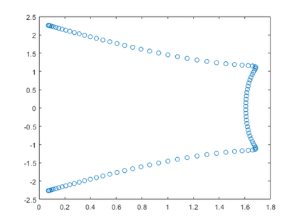
grcar

Joe Grcar会给我们一个有趣的图表。

dbtype7:10私人/ grcar

J. F. Grcar，线性方程的算子系数法，9%报告SAND89-8691, Sandia国家实验室，Albuquerque, 10% New Mexico, 1989(附录2)。

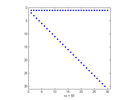
N = 12;Z =画廊“grcar”, n)

Z = 1 1 1 1 0 0 0 0 0 0 0 0 1 1 1 1 1 0 0 0 0 0 0 0 0 1 1 1 1 1 0 0 0 0 0 0 0 0 1 1 1 1 1 0 0 0 0 0 0 0 0 1 1 1 1 1 0 0 0 0 0 0 0 0 1 1 1 1 1 0 0 0 0 0 0 0 0 1 1 1 1 1 0 0 0 0 0 0 0 0 1 1 1 1 1 0 0 0 0 0 0 0 0 1 1 1 1 1 0 0 0 0 0 0 0 0 1 1 1 1 0 0 0 0 0 0 0 0 0 1 1 1 0 0 0 0 0 0 0 0 0 0 1 1

N = 100;Z =画廊“grcar”n);e = eig(Z);情节(e,“o”）

gallery5

你算出的特征值了吗画廊(5)了吗?记住，矩阵是

G

G = -9 11 -21 63 -252 70 -69 141 -421 1684 -575 575 -1149 3451 -13801 3891 -3891 7782 -23345 93365 1024 -1024 2048 -6144 24572

MATLAB说特征值是

e = eig(G)

E = -0.034729401323988 + 0.025790098411744i - 0.025790098411744i 0.013777607600186 + 0.040110258133935i 0.041903587448437 + 0.000000000000000i

但是，看看的幂G。自G有整数项(它是波希米亚的)，它的项可以不舍入计算。四次方是

G ^ 4

Ans = 0 0 0 0 0 0 -84 168 -420 1344 -5355 568 -1136 2840 -9088 36210 -3892 7784 -19460 62272 -248115 -1024 2048 -5120 16384 -65280

五次方是

G ^ 5

Ans = 0 0 0 0 0 0 0 0 0 0 0 0 0 0 0 0

所有的零。

的Cayley-Hamilton定理告诉我们特征多项式必须是

x ^ 5

特征值，这个多项式的唯一根，是零，代数多重性为5。

MATLAB有效地求解

x ^ 5=舍入

因此计算出的特征值来自

x=(凑整)^ (1/5)

很难将它们识别为零的扰动。

获取MATLAB代码

使用MATLAB®R2018b发布