Exploring the Data Set

该示例使用来自Derisi等人的酵母中基因表达的微阵列表达的数据。1997 [1]。作者使用DNA微阵列研究几乎所有基因的时间基因表达酿酒酵母酿酒酵母在代谢从发酵到呼吸的转变期间。在辅助偏移期间在七个时间点测量表达水平。可以从基因表达式omnibus网站下载完整数据集，http://www.ncbi.nlm.nih.gov/geo/query/acc.cgi?acc=GSE28。

该MAT-fileyeastdata.matcontains the expression values (log2 of ratio ofch2dn_mean.和ch1dn_mean.）从实验中的七个时间步骤，基因的名称和测量表达水平的时间阵列。

loadyeastdata.mat

要了解您可以使用的数据的大小numel（基因）为了显示数据集中包含多少个基因。

numel（基因）

ans = 6400.

You can access the genes names associated with the experiment by indexing the variable基因那a cell array representing the gene names. For example, the 15th element in基因是yal054c。这表示变量的第15行yeastvaluescontains expression levels for YAL054C.

基因{15}

ans ='yal054c'

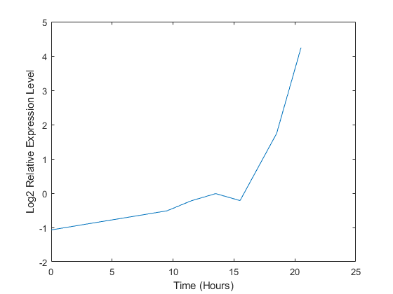
A simple plot can be used to show the expression profile for this ORF.

情节（次，yeastvalues（15，:)）xlabel（'Time (Hours)'）;ylabel（'log2相对表达水平'）;

您还可以绘制实际表达式比率，而不是log2变换的值。

情节(*,2。^yeastvalues(15,:)) xlabel('Time (Hours)'）;ylabel（“相对表达水平”）;

与该ORF，ACS1相关的基因似乎在辅助偏移期间强烈上调。您可以通过在同一图中绘制多条线来将该基因的表达与其他基因的表达进行比较。

保持上情节(*,2。^yeastvalues(16:26,:)') xlabel('Time (Hours)'）;ylabel（“相对表达水平”）;标题（'个人资料表达级别'）;

过滤基因

Typically, a gene expression dataset includes information corresponding to genes that do not show any interesting changes during the experiment. To make it easier to find the interesting genes, you can reduce the size of the data set to some subset that contains only the most significant genes.

如果您浏览基因列表，您将看到几个标记为的斑点'EMPTY'。这些是阵列上的空斑点，而它们可能具有与它们相关联的数据，因为此示例的目的，您可以考虑这些要点是噪声。可以使用这些点使用Strcmp.函数并从具有索引命令的数据集中删除。

emptyspots = strcmp（'EMPTY'，基因）;yeastvalues（空虚，:) = [];基因（Everyspots）= [];numel（基因）

ans = 6314

还有在数据集中看到的几个位置，其中表达级别被标记为NaN。这表明在特定时间步骤中没有收集数据。处理这些缺失值的一种方法是使用时间随时间使用特定基因的均值或数据的平均值或中位数来施加它们。此示例使用较少的严格方法，即仅丢弃未测量一个或多个表达水平的任何基因的数据。功能isnan.用于识别具有缺失数据的基因，使用索引命令用于删除具有缺失数据的基因。

纳丁德=任何（Isnan（yeastvalues），2）;yeastvalues（纳丁德，:) = [];基因（Naninindes）= [];numel（基因）

ANS = 6276.

If you were to plot the expression profiles of all the remaining profiles, you would see that most profiles are flat and not significantly different from the others. This flat data is obviously of use as it indicates that the genes associated with these profiles are not significantly affected by the diauxic shift; however, in this example, you are interested in the genes with large changes in expression accompanying the diauxic shift. You can use filtering functions in the Bioinformatics Toolbox™ to remove genes with various types of profiles that do not provide useful information about genes affected by the metabolic change.

你可以使用GenevarFilter.滤除随时间差异小的基因的功能。该函数返回与变量相同大小的逻辑阵列（即掩码）基因与相对应的行yeastvalueswith variance greater than the 10th percentile and zeros corresponding to those below the threshold. You can use the mask to index into the values and remove the filtered genes.

面具= Genevarfilter（yeastvalues）;yeastvalues = yeastvalues（面具，:);基因=基因（面膜）;numel（基因）

ans = 5648.

功能genelowvalfilterremoves genes that have very low absolute expression values. Note that these filter functions can also automatically calculate the filtered data and names, so it is not necessary to index the original data using the mask.

[掩盖，酵母，基因] = Genelowvalfilter（酵母，基因，基因，'absval'，log2（3））;numel（基因）

ANS = 822.

Finally, you can use the functiongeneentropyfilter删除其配置文件具有低熵的基因，例如数据的第15位熵级别。

[面膜，酵母，基因] =基因裂解（酵母，基因，'proctile'15);numel（基因）

ANS = 614.

Cluster Analysis

Now that you have a manageable list of genes, you can look for relationships between the profiles using some different clustering techniques from the Statistics and Machine Learning Toolbox™. For hierarchical clustering, the functionPdist.计算配置文件之间的成对距离和连锁创建分层群集树。

corrdist = pdist（yeastvalues，'corr'）;clustertree =链接（corrdist，'平均'）;

该簇function calculates the clusters based on either a cutoff distance or a maximum number of clusters. In this case, themaxclust选项用于识别16个不同的群集。

clusters = cluster（clustertree，'maxclust'那16);

这些簇中的基因的谱可以使用简单的环路绘制在一起子图命令。

figureforc = 1:16子图（4,4，c）;plot(times,yeastvalues((clusters == c),:)'); axis紧endsuptitle（'配置文件的分层群集'）;

该统计和机器学习工具箱also has a K-means clustering function. Again, sixteen clusters are found, but because the algorithm is different these will not necessarily be the same clusters as those found by hierarchical clustering.

初始化随机数生成器的状态，以确保由这些命令生成的图形匹配此示例的HTML版本中的图。

RNG（'默认'）;[CIDX，CTRS] = kmeans（yeastvalues，16，'dist'那'corr'那'rep'，5，'disp'那'final'）;figureforc = 1:16子图（4,4，c）;图（次数，yeastvalues（（cidx == c），:)'）;轴紧endsuptitle（'K-Means Clustering of Profiles'）;

复制1,21迭代，距离总和= 23.4699。复制2,22迭代，距离总和= 23.5615。复制3,10次迭代，距离总和= 24.823。复制4,28迭代，距离总和= 23.4501。复制5,19迭代，距离总和= 23.5109。最佳距离总和= 23.4501

你可以绘制质心而不是绘制所有配置文件。

figureforc = 1:16子图（4,4，c）;plot(times,ctrs(c,:)'); axis紧轴关闭endsuptitle（'K-Means Clustering of Profiles'）;

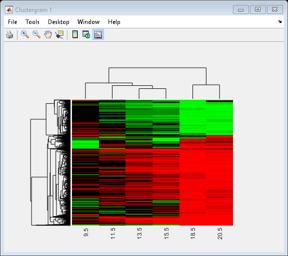
你可以使用clustergram功能要从分层聚类的输出中创建表达式的热图和树木图。

cgObj = clustergram(yeastvalues(:,2:end),'rowlabels'，基因，'columnlabels'，次（2：结束））;

主要成分分析

主组件分析（PCA）是一种有用的技术，可用于降低大数据集的维度，例如微阵列。PCA也可用于在嘈杂数据中找到信号。功能mapcaplot.计算数据集的主要组成部分并创建结果的散点图。您可以交互方式从其中一个绘图中选择数据点，并且这些点在另一个绘图中自动突出显示。这使您可以同时可视化多个维度。

H = MapCaplot（酵母值，基因）;

请注意，前两个主要成分的分数的散点图表明有两个不同的区域。这不是出乎意料的，因为过滤过程删除了具有低方差或低信息的许多基因。这些基因已经出现在散点图的中间。

如果要查看主组件的值，则PC.a统计信息和机器学习工具箱中的功能用于计算数据集的主组件。

[PC，Zscores，PCVARS] = PCA（yeastValues）;

第一个输出，PC.，是一个主要成分的矩阵yeastvaluesdata. The first column of the matrix is the first principal component, the second column is the second principal component, and so on. The second output,ZScores.，包括主成分分数，即主要成分空间中的酵母值的代表。第三个输出，PCVARS.，包含主成分差异，这可以测量每个主组件的数据算法的数量。

很明显，第一个主要成分占模型中的大部分方差。您可以计算每个组件的方差的确切百分比，如下所示。

pcvars./sum(pcvars）* 100

ans = 79.8316 9.5858 4.0781 2.6486 2.1723 0.9747 0.7089

这意味着差异的差异占前两个主要成分的差异。你可以使用浓汤命令查看差异的累积总和。

Cumsum（PCVars./sum（PCVARS）* 100）

ANS = 79.8316 89.4174 93.4955 96.1441 98.3164 99.2911 100.0000

如果您希望在绘制主组件的绘图方面有更多的控制，可以使用分散function.

figure scatter(zscores(:,1),zscores(:,2)); xlabel('第一个主要成分'）;ylabel（'第二个主要成分'）;标题（'主成分散点图'）;

创建散点图的替代方法是函数g箭偶from the Statistics and Machine Learning Toolbox.g箭偶creates a grouped scatter plot where points from each group have a different color or marker. You can useclusterdata.那or any other clustering function, to group the points.

图PCClusters = ClusterData（Zscores（：，1：2），'maxclust'，8，'连锁'那'av'）;g箭偶(zscores(:,1),zscores(:,2),pcclusters) xlabel('第一个主要成分'）;ylabel（'第二个主要成分'）;标题（“主要成分散射块与彩色簇”）;

自组织地图

If you have the Deep Learning Toolbox™, you can use a self-organizing map (SOM) to cluster the data.

％检查是否安装了深度学习工具箱if~exist(which('selforgmap'）那'文件'）disp('此示例的自组织地图部分需要深度学习工具箱。）返回end

该selforgmap函数创建一个新的SOM网络对象。此示例将使用前两个主组件生成一个索峰。

p = zscores（：，1：2）';net = selforgmap（[4 4]）;

使用默认参数列车。

净=火车（网，P）;

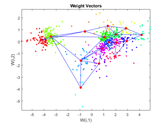
采用Plotsom.在数据的散点图上显示网络。请注意，SOM算法使用随机起始点，因此结果将从运行运行时变化。

图绘图（p（1，:)，p（2，:)，'。G'那'Markersize'，20）持有上Plotsom（net.iw {1,1}，net.layers {1} .distans）持有关闭

您可以通过查找数据集中的每个点来分配使用SOM的群集。

distances = dist(P',net.IW{1}'); [d,cndx] = min(distances,[],2);% cndx contains the cluster index图g箭偶（p（1，:)，p（2，:)，cndx）;传说关闭; hold上Plotsom（net.iw {1,1}，net.layers {1} .distans）;保持关闭

关all figures and apps.

关（'all'）;删除（cgobj）;删除（h）;nntraintool（'关'）;

参考资料

[1] DeRisi, J.L., Iyer, V.R. and Brown, P.O., "Exploring the metabolic and genetic control of gene expression on a genomic scale", Science, 278(5338):680-6, 1997.