Decoupling Controller for a Distillation Column
This example shows how to uselooptuneto decouple the two main feedback loops in a distillation column.
Distillation Column Model
This example uses a simple model of the distillation column shown below.

Figure 1: Distillation Column
In the so-called LV configuration, the controlled variables are the concentrationsyDandyBof the chemicalsD(tops) andB(底部)the manipulated variables are the refluxLand boilupV. This process exhibits strong coupling and large variations in steady-state gain for some combinations of L and V. For more details, see Skogestad and Postlethwaite,Multivariable Feedback Control.
The plant is modeled as a first-order transfer function with inputsL,Vand outputsyD,yB:

The unit of time is minutes (all plots are in minutes, not seconds).
s = tf('s'); G = [87.8 -86.4 ; 108.2 -109.6]/(75*s+1); G.InputName = {'L','V'}; G.OutputName = {'yD','yB'};
Control Architecture
The control objectives are as follows:
Independent control of the tops and bottoms concentrations by ensuring that a change in the tops setpoint
Dsphas little impact on the bottoms concentrationBand vice versaResponse time of about 4 minutes with less than 15% overshoot
Fast rejection of input disturbances affecting the effective reflux
Land boilupV
To achieve these objectives we use the control architecture shown below. This architecture consists of a static decoupling matrixDMin series with two PI controllers for the refluxLand boilupV.
open_system('rct_distillation')

Controller Tuning in Simulink with LOOPTUNE
Thelooptunecommand provides a quick way to tune MIMO feedback loops. When the control system is modeled in Simulink, you just specify the tuned blocks, the control and measurement signals, and the desired bandwidth, andlooptuneautomatically sets up the problem and tunes the controller parameters.looptuneshapes the open-loop response to provide integral action, roll-off, and adequate MIMO stability margins.
Use theslTunerinterface to specify the tuned blocks, the controller I/Os, and signals of interest for closed-loop validation.
ST0 = slTuner('rct_distillation',{'PI_L','PI_V','DM'});% Signals of interestaddPoint (ST0, {'r','dL','dV','L','V','y'})
Set the control bandwidth by specifying the gain crossover frequency for the open-loop response. For a response time of 4 minutes, the crossover frequency should be approximately 2/4 = 0.5 rad/min.
wc = 0.5;
UseTuningGoalobjects to specify the remaining control objectives. The response to a step command should have less than 15% overshoot. The response to a step disturbance at the plant input should be well damped, settle in less than 20 minutes, and not exceed 4 in amplitude.
OS = TuningGoal.Overshoot('r','y',15); DR = TuningGoal.StepRejection({'dL','dV'},'y',4,20);
Next uselooptuneto tune the controller blocksPI_L,PI_V, andDMsubject to the disturbance rejection requirement.
Controls = {'L','V'}; Measurements ='y'; [ST,gam,Info] = looptune(ST0,Controls,Measurements,wc,OS,DR);
Final: Peak gain = 0.983, Iterations = 55 Achieved target gain value TargetGain=1.
The final value is near 1 which indicates that all requirements were met. Useloopviewto check the resulting design. The responses should stay outside the shaded areas.
figure('Position',[0,0,1000,1200]) loopview(ST,Info)

UsegetIOTransferto access and plot the closed-loop responses from reference and disturbance to the tops and bottoms concentrations. The tuned responses show a good compromise between tracking and disturbance rejection.
figure Ttrack = getIOTransfer(ST,'r','y'); step(Ttrack,40), grid, title('Setpoint tracking')

Treject = getIOTransfer(ST,{'dV','dL'},'y'); step(Treject,40), grid, title('Disturbance rejection')

Comparing the open- and closed-loop disturbance rejection characteristics in the frequency domain shows a clear improvement inside the control bandwidth.
clf, sigma(G,Treject), grid title('Principal gains from input disturbances to outputs') legend('Open-loop','Closed-loop')

Adding Constraints on the Tuned Variables
Inspection of the controller obtained above shows that the second PI controller has negative gains.
getBlockValue(ST,'PI_V')
ans = 1 Kp + Ki * --- s with Kp = -4.94, Ki = -0.684 Name: PI_V Continuous-time PI controller in parallel form.
This is due to the negative signs in the second input channels of the plant . In addition, the tunable elements are over-parameterized because multiplying
DMby two and dividing the PI gains by two does not change the overall controller. To address these issues, fix the (1,1) entry ofDMto 1 and the (2,2) entry to -1.
DM = getBlockParam(ST0,'DM'); DM.Gain.Value = diag([1 -1]); DM.Gain.Free = [false true;true false]; setBlockParam(ST0,'DM',DM)
Re-tune the controller for the reduced set of tunable parameters.
[ST,gam,Info] = looptune(ST0,Controls,Measurements,wc,OS,DR);
Final: Peak gain = 0.998, Iterations = 93 Achieved target gain value TargetGain=1.
The step responses look similar but the values ofDMand the PI gains are more suitable for implementation.
figure('Position', 0700350年,[0])次要情节(121)Ttrack = getIOTransfer(ST,'r','y'); step(Ttrack,40), grid, title('Setpoint tracking') subplot(122) Treject = getIOTransfer(ST,{'dV','dL'},'y'); step(Treject,40), grid, title('Disturbance rejection')

showTunable(ST)
Block 1: rct_distillation/PI_L = 1 Kp + Ki * --- s with Kp = 16.4, Ki = 2.17 Name: PI_L Continuous-time PI controller in parallel form. ----------------------------------- Block 2: rct_distillation/PI_V = 1 Kp + Ki * --- s with Kp = 12.9, Ki = 1.71 Name: PI_V Continuous-time PI controller in parallel form. ----------------------------------- Block 3: rct_distillation/DM = D = u1 u2 y1 1 -0.7713 y2 1.254 -1 Name: DM Static gain.
Equivalent Workflow in MATLAB
If you do not have a Simulink model of the control system, you can use LTI objects and Control Design blocks to create a MATLAB representation of the following block diagram.

Figure 2: Block Diagram of Control System
First parameterize the tunable elements using Control Design blocks. Use thetunableGainobject to parameterizeDMand fixDM(1,1)=1andDM(2,2)=-1. This creates a 2x2 static gain with the off-diagonal entries as tunable parameters.
DM = tunableGain('Decoupler',diag([1 -1])); DM.Gain.Free = [false true;true false];
Similarly, use thetunablePIDobject to parameterize the two PI controllers:
PI_L = tunablePID('PI_L','pi'); PI_V = tunablePID('PI_V','pi');
Next construct a modelC0of the controller in Figure 2.
C0 = blkdiag(PI_L,PI_V) * DM * [eye(2) -eye(2)];% Note: I/O names should be consistent with those of GC0。InputName = {'Dsp','Bsp','yD','yB'}; C0.OutputName = {'L','V'};
Now tune the controller parameters withlooptuneas done previously.
% Crossover frequencywc = 0.5;% Overshoot and disturbance rejection requirementsOS = TuningGoal.Overshoot({'Dsp','Bsp'},{'yD','yB'},15); DR = TuningGoal.StepRejection({'L','V'},{'yD','yB'},4,20);% Tune controller gains[~,C] = looptune(G,C0,wc,OS,DR);
Final: Peak gain = 0.995, Iterations = 59 Achieved target gain value TargetGain=1.
To validate the design, close the loop with the tuned compensatorCand simulate the step responses for setpoint tracking and disturbance rejection.
Tcl = connect(G,C,{'Dsp','Bsp','L','V'},{'yD','yB'}); figure('Position', 0700350年,[0])次要情节(121)Ttrack = Tcl(:,[1 2]); step(Ttrack,40), grid, title('Setpoint tracking') subplot(122) Treject = Tcl(:,[3 4]); Treject.InputName = {'dL','dV'}; step(Treject,40), grid, title('Disturbance rejection')

The results are similar to those obtained in Simulink.
See Also
looptune|looptune(slTuner)(Simulink Control Design)
Related Topics
Select a Web Site
Choose a web site to get translated content where available and see local events and offers. Based on your location, we recommend that you select:.
Selectweb siteYou can also select a web site from the following list:
Americas
- América Latina(Español)
- Canada(English)
- United States(English)
Europe
- Belgium(English)
- Denmark(English)
- Deutschland(Deutsch)
- España(Español)
- Finland(English)
- France(Français)
- Ireland(English)
- Italia(Italiano)
- Luxembourg(English)
- Netherlands(English)
- Norway(English)
- Österreich(Deutsch)
- Portugal(English)
- Sweden(English)
- Switzerland
- United Kingdom(English)