Load and Preprocess Data

Load the data from the XLS spreadsheet. Use the'basic'command option for non-Windows® platforms.

创建一个变量Nthat has all the numeric data in one array.

n = xlsread（'Engine_Data_si_na_2l_i4.xls'那'SI NA 2L I4'那''那'basic'）;

Extract from the variableNthe columns of interest.

SPEED = n(:,2); LOAD_CMD = n(:,3); LOAD = n(:,8); BSFC = n(:,22);

Process the data before fitting, to pick out the minimum BSFC values from each sweep. The data points are organized in sweeps on speed/load.

获取速度/加载站点的列表：

SL =唯一（[速度，load_cmd]，'行'）;nruns =尺寸（sl，1）;

对于每个速度/加载站点，在站点上找到数据并提取实际测量的负载和最小BSFC。

minBSFC = zeros( nRuns, 1 ); Load = zeros( nRuns, 1 ); Speed = zeros( nRuns, 1 );对于i = 1:nRuns idx = SPEED == SL(i,1) & LOAD_CMD == SL(i,2); minBSFC(i) = min( BSFC(idx) ); Load(i) = mean( LOAD(idx) ); Speed(i) = mean( SPEED(idx) );结束

适合曲面

将燃料效率的表面符合预处理数据。

F1 = FIT（[速度，装载]，MINBSFC，'Lowess'那'正常化'那'上'）

Locally weighted smoothing linear regression: f1(x,y) = lowess (linear) smoothing regression computed from p where x is normalized by mean 3407 and std 1214 and where y is normalized by mean 0.5173 and std 0.1766 Coefficients: p = coefficient structure

情节适合

绘图（F1，[速度，装载]，MINBSFC）;Xlabel（'速度[rpm]'）;ylabel（'Load [%]'）;Zlabel（'最小bsfc [g / kwh]'）;

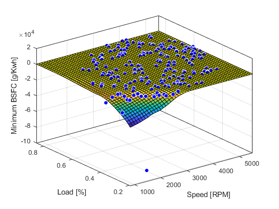
删除问题点

查看结果的情节。

There are points where BSFC is negative because this data is generated by an engine simulation.

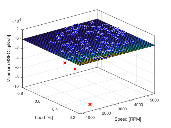
通过保持范围的点[0，INF]来删除这些问题数据点。

OUT = EXCLUDEDATA（速度，MINBSFC，'范围'，[0，INF]）;F2 = FIT（[速度，装载]，MINBSFC，'Lowess'那......'正常化'那'上'那'Exclude'，出）

局部加权平滑线性回归：F2（x，y）=从p的p计算的ZHOSE（线性）平滑回归，其中X由平均3443和STD 1187归一化，其中Y通过平均值为0.521和STD 0.175系数归一化：P =系数结构

Plot the new fit. Note that the excluded points are plotted as red crosses.

绘图（F2，[速度，装载]，MINBSFC，'Exclude'，出）;Xlabel（'速度[rpm]'）;ylabel（'Load [%]'）;Zlabel（'最小bsfc [g / kwh]'）;

放大

Zoom in on the part of the z-axis of interest.

zlim([0, max( minBSFC )])

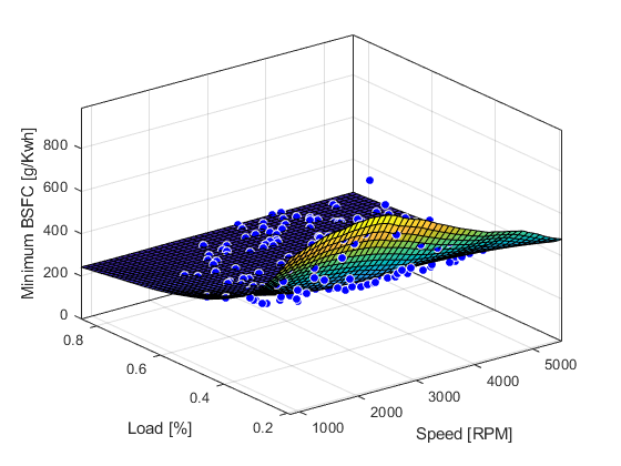
您希望有效地操作发动机，因此创建一个轮廓图以查看BSFC低的区域。使用绘图函数，并指定名称/值参数对'style','Contour'。

绘图（F2，[速度，装载]，MINBSFC，'Exclude'，出，'风格'那'Contour'）;Xlabel（'速度[rpm]'）;ylabel（'Load [%]'）;彩色栏

从表面创建一个表

Generate a table by evaluating the modelF2在一个点的网格上。

为表断点创建变量。

速度消耗= linspace( 1000, 5500, 17 ); loadbreakpoints = linspace( 0.2, 0.8, 13 );

To generate values for the table, evaluate the model over a grid of points.

[tSpeed, tLoad] = meshgrid( speedbreakpoints, loadbreakpoints ); tBSFC = f2( tSpeed, tLoad );

在命令行中检查表的行和列。

TBSFC（1：2：结束，1：2：结束）

ANS =列1至7 722.3280 766.7608 779.4296 757.4574 694.5378 624.4095 576.5235 503.9880 499.9201 481.7240 458.2803 427.7338 422.1099 412.1624 394.7579 364.3421 336.1811 330.1550 329.1635 328.1810 329.1144 333.7740 307.7736 295.1777 291.2068 290.3637 290.0173 287.8672 295.9729 282.7567 273.8287 270.8869 269.8485 271.0547 270.5502 273.7512 264.5167 259.7631 257.9215 256.9350 258.3228 258.6638 251.5652 247.6746247.2747 247。

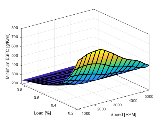
Plot the Table Against the Original Model

The grid on the model surface shows the table breakpoints.

h = plot（f2）;H.edgecolor ='没有';保持onmesh( tSpeed, tLoad, tBSFC,......'LineStyle'那' - '那'行宽'2，'Edgecolor'那'k'那......'facecholor'那'没有'那'Facealpha'，1）;保持offXlabel（'速度[rpm]'）;ylabel（'Load [%]'）;Zlabel（'最小bsfc [g / kwh]'）;

Check the Table Accuracy

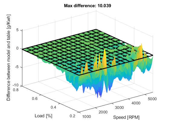
View the difference between the model and the table by plotting the difference between them on a finer grid. Then, use this difference in prediction accuracy between the table and the model to determine the most efficient table size for your accuracy requirements.

The following code evaluates the model over a finer grid and plots the difference between the model and the table.

[tfspeed，tfload] = meshgrid（......linspace( 1000, 5500, 8*17+1 ),......linspace (0.2, 0.8, 8 * 13 + 1));tfBSFC_model = f2 (tfSpeed, tfLoad ); tfBSFC_table = interp2( tSpeed, tLoad, tBSFC, tfSpeed, tfLoad,'线性'）;tfdiff = tfbsfc_model  -  tfbsfc_table;冲浪（TFSPEED，TFLOAD，TFDIFF，'LineStyle'那'没有'）;保持on网格（TSPEED，Tload，零（尺寸（TBSFC）），......'LineStyle'那' - '那'行宽'2，'Edgecolor'那'k'那......'facecholor'那'没有'那'Facealpha'，1）;保持offaxistightXlabel（'速度[rpm]'）;ylabel（'Load [%]'）;Zlabel（'模型和表之间的区别[g / kwh]'）;标题（Sprintf（'最大差异：％g'，max（abs（tfdiff（:)））））;

Create a Table Array Including Breakpoint Values

After creating a table by evaluating a model fit over a grid of points, it can be useful to export your table data from MATLAB. Before exporting, create a table array that includes the breakpoint values in the first row and column. The following command reshapes your data to this table format:

table = [ {'Load\Speed'}, num2cell(speedbreakpoints(:).' ) num2cell(loadbreakpoints (:) ), num2cell( tBSFC ) ];

Export Table to Spreadsheet File

你可以使用xlswrite.function to export your table data to a new Excel Spreadsheet. Execute the following command to create a spreadsheet file.

xlswrite（'tabledata.xlsx'那table )

Create a Lookup Table Block

如果您有Simulink金宝app™软件，则可以如下创建查找表块。执行以下代码以尝试。

1. Create a model with a 2-D Lookup Table block.

金宝appsimulink new_system（'my_model'）Open_System（'my_model'）add_block('金宝appSimulink / Lookup表/ 2-D查找表'那'my_model/surfaceblock'）

2.使用速度断点，加载断点和查找表填充查找表。

set_param('my_model/surfaceblock'那......'BreakpointsForDimension1'那'loadbreakpoints'那......'BreakpointsForDimension2'那'speedbreakpoints'那......'表'那'tbsfc'）;

3. Examine the populated Lookup Table block.