Discrete-Time Narendra-Li Benchmark System

The discrete-time equations of the Narendra-Li system are:

x1(t+Ts) = (x1(t)/(1+x1(t)^2)+p(1))*sin(x2(t)) x2(t+Ts) = x2(t)*cos(x2(t)) + x1(t)*exp(-(x1(t)^2+x2(t)^2)/p(2)) + u(t)^3/(1+u(t)^2+p(3)*cos(x1(t)+x2(t))

y(t) = x1(t)/(1+p(4)*sin(x2(t))+p(5)*sin(x1(t)))

其中x1（t）和x2（t）是状态，U（t）输入信号，y（t）输出信号和p参数向量，其中具有5个元素。

Idnlgrey离散时间Narendra-Li模型

从idnlgrey模型文件的角度来看，连续和离散时间系统之间没有区别。因此，Narendra-Li模型文件必须返回状态更新向量DX和输出Y，并且应该取t（时间），x（状态向量），u（输入），p（参数）和varargin作为输入参数：

function [dx, y] = narendrali_m(t, x, u, p, varargin) %NARENDRALI_M A discrete-time Narendra-Li benchmark system.

％输出方程。Y = X（1）/（1 + P（4）* SIN（x（2）））+ x（2）/（1 + P（5）* SIN（x（1）））;

％状态方程。dx = [（x（1）/（1 + x（1）^ 2）+ p（1））* sin（x（2））;...％状态1. x（2）* cos（x（2））+ x（1）* exp（ - （x（1）^ 2 + x（2）^ 2）/ p（2））。..％状态2. + U（1）^ 3 /（1 + U（1）^ 2 + P（3）* cos（x（1）+ x（2））））...];

请注意，我们在此选择将所有5个参数融为一个参数向量，其中I：Th元素在通常的Matlab方式中引用，即通过P（i）。

使用此模型文件作为基础，我们接下来创建反映建模情况的idnlgrey对象。这里值得强调是通过Ts（= 1秒）的正值来指定模型的离散性。请注意，参数仅保存一个元素，5×1参数向量，并且setPar用于指定此向量的所有组件都是严格正面的。

FileName ='narendrali_m';％文件描述模型结构。Order = [1 1 2];% Model orders [ny nu nx].参数= {[1.05;7.00;0.52;0.52;0.48]};% True initial parameters (a vector).InitialStates = zeros(2, 1);% Initial value of initial states.Ts = 1;% Time-discrete system with Ts = 1s.nlgr = idnlgrey(FileName, Order, Parameters, InitialStates, Ts,'Name',...'离散时间Narendra-Li基准系统',...'TimeUnit',s）;nlgr = setpar(nlgr,'Minimum', {eps(0)*ones(5, 1)});

A summary of the entered Narendra-Li model structure is obtained through the PRESENT command:

present(nlgr);

nlgr = Discrete-time nonlinear grey-box model defined by 'narendrali_m' (MATLAB file): x(t+Ts) = F(t, u(t), x(t), p1) y(t) = H(t, u(t), x(t), p1) + e(t) with 1 input(s), 2 state(s), 1 output(s), and 5 free parameter(s) (out of 5). Inputs: u(1) (t) States: Initial value x(1) x1(t) xinit@exp1 0 (fixed) in [-Inf, Inf] x(2) x2(t) xinit@exp1 0 (fixed) in [-Inf, Inf] Outputs: y(1) (t) Parameters: Value p1(1) p1 1.05 (estimated) in ]0, Inf] p1(2) 7 (estimated) in ]0, Inf] p1(3) 0.52 (estimated) in ]0, Inf] p1(4) 0.52 (estimated) in ]0, Inf] p1(5) 0.48 (estimated) in ]0, Inf] Name: Discrete-time Narendra-Li benchmark system Sample time: 1 seconds Status: Created by direct construction or transformation. Not estimated. More information in model's "Report" property.

Input-Output Data

Two input-output data records with 300 samples each, one for estimation and one for validation purposes, are available. The input vector used for both these records is the same, and was chosen as a sum of two sinusoids:

u(t) = sin(2*pi*t/10) + sin(2*pi*t/25)

t = 0, 1,……, 299秒。我们创建两个差异erent IDDATA objects to hold the two data records, ze for estimation and zv for validation purposes.

load(fullfile(matlabroot,'toolbox','ident','Iddemos','data','narendralidata')); ze = iddata(y1, u, Ts,'tstart', 0,'Name','Narendra-Li估计数据',...'ExperimentName','ze'）;ZV.= iddata(y2, u, Ts,'tstart', 0,'Name','Narendra-Li validation data',...'ExperimentName','ZV'）;

The input-output data that will be used for estimation are shown in a plot window.

数字（'Name', ze.Name); plot(ze);

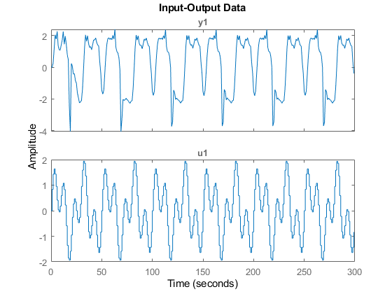
Figure 1:Input-output data from a Narendra-Li benchmark system.

初始Narendra-Li模型的表现

Let us now use COMPARE to investigate the performance of the initial Narendra-Li model. The simulated and measured outputs for泽andZV.生成，并适合泽默认情况下显示。使用绘图上下文菜单切换数据实验ZV.. The fit is not that bad for either dataset (around 74 %). Here we should point out that COMPARE by default estimates the initial state vector, in this case one initial state vector for泽另一个是ZV..

compare(merge(ze, zv), nlgr);

Figure 2:真正输出与初始Narendra-Li模型的模拟输出之间的比较。

%%4通过查看通过PE获得的预测误差来实现％，我们意识到％初始Narendra-Li模型显示了一些系统和周期性的差异% as compared to the true outputs.pe（合并（ze，zv），nlgr）;

Figure 3:Prediction errors obtained with the initial Narendra-Li model. Use context menu to switch between experiments.

Parameter Estimation

为了减少系统差异，我们使用NLGreyest估计Narendra-Li模型结构的所有5个参数。基于仅估计数据集ZE执行估计。

opt = nlgreyestoptions（'Display','在'）;nlgr = nlgreyest（ze，nlgr，选择）;

Performance of the Estimated Narendra-Li Model

比较再次用于调查估计模型的性能，但这次我们使用模型的内部存储的初始状态向量（对于两个实验的初始状态矢量）而没有任何初始状态矢量估计。

clf opt = compareOptions('InitialCondition','m'）;比较（合并（ZE，ZV），NLGR，选择）;

Figure 4:Comparison between true outputs and the simulated outputs of the estimated Narendra-Li model.

The improvement after estimation is significant, which perhaps is best illustrated through a plot of the prediction errors:

figure; pe(merge(ze, zv), nlgr);

Figure 5:Prediction errors obtained with the estimated Narendra-Li model.

估计的Narendra-Li模型的建模功率也通过渣油提供的相关性分析证实了：

数字（'Name', [nlgr.Name': residuals of estimated model']); resid(zv, nlgr);

Figure 6:Residuals obtained with the estimated Narendra-Li model.

实际上，获得的模型参数也非常接近用于生成真实模型输出的：

disp(' True Estimated parameter vector'）;ptrue = [1;8;0.5;0.5;0.5];FPRINTF（' %1.4f %1.4f\n'，[ptrue';getPvec（nlgr）']）;

True Estimated parameter vector 1.0000 1.0000 8.0000 8.0082 0.5000 0.5003 0.5000 0.4988 0.5000 0.5018

Some additional model quality results (loss function, Akaike's FPE, and the estimated standard deviations of the model parameters) are next provided via the PRESENT command:

present(nlgr);

nlgr = Discrete-time nonlinear grey-box model defined by 'narendrali_m' (MATLAB file): x(t+Ts) = F(t, u(t), x(t), p1) y(t) = H(t, u(t), x(t), p1) + e(t) with 1 input(s), 2 state(s), 1 output(s), and 5 free parameter(s) (out of 5). Inputs: u(1) u1(t) States: Initial value x(1) x1(t) xinit@exp1 0 (fixed) in [-Inf, Inf] x(2) x2(t) xinit@exp1 0 (fixed) in [-Inf, Inf] Outputs: y(1) y1(t) Parameters: Value Standard Deviation p1(1) p1 0.999993 0.0117615 (estimated) in ]0, Inf] p1(2) 8.00821 0.885988 (estimated) in ]0, Inf] p1(3) 0.500319 0.0313092 (estimated) in ]0, Inf] p1(4) 0.498842 0.264806 (estimated) in ]0, Inf] p1(5) 0.501761 0.30998 (estimated) in ]0, Inf] Name: Discrete-time Narendra-Li benchmark system Sample time: 1 seconds Status: Termination condition: Change in parameters was less than the specified tolerance.. Number of iterations: 16, Number of function evaluations: 17 Estimated using Solver: FixedStepDiscrete; Search: lsqnonlin on time domain data "Narendra-Li estimation data". Fit to estimation data: 99.44% FPE: 9.23e-05, MSE: 8.927e-05 More information in model's "Report" property.

至于连续输入输出系统,它是also possible to use STEP for discrete-time input-output systems. Let us do this for two different step levels, 1 and 2:

数字（'Name', [nlgr.Name': step responses of estimated model']); t = (-5:50)'; step(nlgr,'b'，t，stepdataOptions（'stepamplitute',1)); line(t, step(nlgr, t, stepDataOptions('stepamplitute',2)),'color','G'）;网格on; legend('0 -> 1','0  - > 2','Location','NorthWest'）;

Figure 7:用估计的Narendra-Li模型获得的步骤响应。

We conclude this example by comparing the performance of the estimated IDNLGREY Narendra-Li model with some basic linear models. The fit obtained for the latter models are considerably lower than what is returned for the estimated IDNLGREY model.

nk = delayest(ze); arx22 = arx(ze, [2 2 nk]);% Second order linear ARX model.arx33 = arx(ze, [3 3 nk]);％三阶线性ARX模型。arx44 = arx(ze, [4 4 nk]);% Fourth order linear ARX model.oe22 = oe(ze, [2 2 nk]);% Second order linear OE model.OE33 = OE（ze，[3 3 nk]）;% Third order linear OE model.OE44 = OE（ZE，[4 4 NK]）;% Fourth order linear OE model.CLF图= GCF;POS = FIG.POST;fig.Position = [POS（1：2）* 0.7，POS（3）* 1.3，POS（4）* 1.3];比较（zv，nlgr，'b', arx22,'m-'，ARX33，'M：'，ARX44，'m--',...oe22,'G-'，OE33，'g:', oe44,'G - '）;

Figure 8:真正输出与估计Narendra-Li模型的模拟输出之间的比较。

Conclusions

In this example we have used a fictive discrete-time Narendra-Li benchmark system to illustrate the basics for performing discrete-time IDNLGREY modeling.