Open the Model

Open the Simulink model.

mdl ='Boiler_Demo'; open_system(mdl)

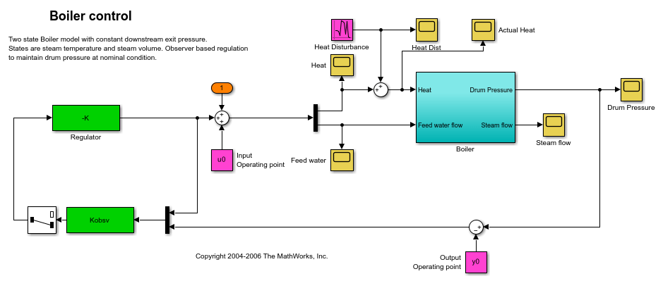
When you open boiler control model the software initializes the controller sizes.u0andy0are set after the operating point computation and are therefore initially set to zero. The observer and regulator are computed during the controller design step and are also initially set to zero.

Find Nominal Operating Point and Linearize Model

模型中定义的初始状态值Simulink model. Using these state values, find the steady-state operating point using thefindopfunction.

Create an operating point specification where the state values are known.

opspec = operspec(mdl); opspec.States(1).Known = 1; opspec.States(2).Known = 1; opspec.States(3).Known = [1;1];

Adjust the operating point specification to indicate that the inputs must be computed and that they are lower-bounded.

opspec.Inputs(1)。Known = [0;0];% Inputs unknownopspec.Inputs(1)。最小值= (0;0];% Input minimum value

Add an output specification to the operating point specification; this is necessary to ensure that the output operating point is computed during the solution process.

opspec = addoutputspec(opspec,[mdl'/Boiler'],1); opspec.Outputs(1).Known = 0;% Outputs unknownopspec.Outputs(1).Min = 0;% Output minimum value

Compute the operating point, and generate an operating point search report.

[opSS,opReport] = findop(mdl,opspec);

Operating point search report: --------------------------------- opreport = Operating point search report for the Model Boiler_Demo. (Time-Varying Components Evaluated at time t=0) Operating point specifications were successfully met. States: ---------- Min x Max dxMin dx dxMax ___________ ___________ ___________ ___________ ___________ ___________ (1.) Boiler_Demo/Boiler/Steam volume 5.6 5.6 5.6 0 7.8501e-13 0 (2.) Boiler_Demo/Boiler/Temperature 180 180 180 0 -5.9262e-14 0 (3.) Boiler_Demo/Observer/Internal 0 0 0 0 0 0 0 0 0 0 0 0 Inputs: ---------- Min u Max ___________ ___________ ___________ (1.) Boiler_Demo/Input 0 241069.0782 Inf 0 100.1327 Inf Outputs: ---------- Min y Max ________ ________ ________ (1.) Boiler_Demo/Boiler 0 1002.381 Inf

Before linearizing the model around this point, specify the input and output signals for the linear model. First, specify the input points for linearization.

Boiler_io(1) = linio([mdl'/Sum'],1,'input'); Boiler_io(2) = linio([mdl'/Demux'],2,'input');

Next, specify the open-loop output points for linearization.

(mdl Boiler_io (3) = linio ('/Boiler'],1,'openoutput'); setlinio(mdl,Boiler_io);

Find a linear model around the chosen operating point.

Lin_Boiler = linearize(mdl,opSS,Boiler_io);

Finally, using theminrealfunction, make sure that the model is a minimum realization.

Lin_Boiler = minreal(Lin_Boiler);

1 state removed.

Design Regulator and State Observer

Using this linear model, design an LQR regulator and Kalman filter state observer. First, find the controller offsets to make sure that the controller is operating around the chosen linearization point by retrieving the computed operating point.

u0 = opReport.Inputs.u; y0 = opReport.Outputs.y;

Now, design the regulator using thelqryfunction. Tight regulation of the output is required while input variation should be limited.

Q = diag(1e8);% Output regulationR = diag([1e2,1e6]);% Input limitation[K,S,E] = lqry(Lin_Boiler,Q,R);

Design the Kalman state observer using thekalmanfunction. For this example, the main noise source is process noise. The noise enters the system only through one input, hence the form ofGandH.

[A,B,C,D] = ssdata(Lin_Boiler); G = B(:,1); H = 0; QN = 1e4; RN = 1e-1; NN = 0; [Kobsv,L,P] = kalman(ss(A,[B G],C,[D H]),QN,RN);

Simulate Model

Simulate the model for the designed controller.

sim(mdl)

Plot the process input and output signals. The following figure shows the feed water actuation signal in kg/s.

plot(FeedWater.time/60,FeedWater.signals.values) title('Feedwater flow rate [kg/s]'); ylabel('Flow [kg/s]') xlabel('time [min]') gridon

The following plot shows the heat actuation signal in kJ.

plot(Heat.time/60,Heat.signals.values/1000) title('Applied heat [kJ]'); ylabel('Heat [kJ]') xlabel('time [min]') gridon

The next figure shows the heat disturbance in kJ. The disturbance varies by as much as 50% of the nominal heat value.

plot(HeatDist.time/60,HeatDist.signals.values/1000) title('Heat disturbance [kJ]'); ylabel('Heat [kJ]') xlabel('time [min]') gridon

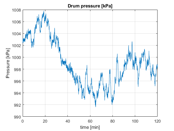
The figure below shows the corresponding drum pressure in kPa. The pressure varies by about 1% of the nominal value even though the disturbance is relatively large.

plot(DrumPressure.time/60,DrumPressure.signals.values) title('Drum pressure [kPa]'); ylabel('Pressure [kPa]') xlabel('time [min]') gridonbdclose(mdl)