Load a multivariate signal by typing the following at the MATLAB^®prompt:

load ex4mwden whos

Usually, only the matrix of dataxis available. Here, we also have the true noise covariance matrix (covar) and the original signals (x_orig). These signals are noisy versions of simple combinations of the two original signals. The first one is “Blocks” which is irregular, and the second is “HeavySine,” which is regular except around time 750. The other two signals are the sum and the difference of the two original signals. Multivariate Gaussian white noise exhibiting strong spatial correlation is added to the resulting four signals, which leads to the observed data stored inx。

Display the original and observed signals by typing

kp = 0; for i = 1:4 subplot(4,2,kp+1), plot(x_orig(:,i)); axis tight; title(['Original signal ',num2str(i)]) subplot(4,2,kp+2), plot(x(:,i)); axis tight; title(['Observed signal ',num2str(i)]) kp = kp + 2; end

The true noise covariance matrix is given by

covar covar = 1.0000 0.8000 0.6000 0.7000 0.8000 1.0000 0.5000 0.6000 0.6000 0.5000 1.0000 0.7000 0.7000 0.6000 0.7000 1.0000

Remove noise by simple multivariate thresholding.

The denoising strategy combines univariate wavelet denoising in the basis where the estimated noise covariance matrix is diagonal with noncentered Principal Component Analysis (PCA) on approximations in the wavelet domain or with final PCA.

First, perform univariate denoising by typing the following to set the denoising parameters:

level = 5; wname = 'sym4'; tptr = 'sqtwolog'; sorh = 's';

Then, set the PCA parameters by retaining all the principal components:

npc_app = 4; npc_fin = 4;

Finally, perform multivariate denoising by typing

x_den = wmulden(x, level, wname, npc_app, npc_fin, tptr, sorh);

Display the original and denoised signals by typing

kp = 0; for i = 1:4 subplot(4,3,kp+1), plot(x_orig(:,i)); set(gca,'xtick',[]); axis tight; title(['Original signal ',num2str(i)]) subplot(4,3,kp+2), plot(x(:,i)); set(gca,'xtick',[]); axis tight; title(['Observed signal ',num2str(i)]) subplot(4,3,kp+3), plot(x_den(:,i)); set(gca,'xtick',[]); axis tight; title(['denoised signal ',num2str(i)]) kp = kp + 3; end

Improve the first result by retaining fewer principal components.

The results are satisfactory. Focusing on the two first signals, note that they are correctly recovered, but the result can be improved by taking advantage of the relationships between the signals, leading to an additional denoising effect.

To automatically select the numbers of retained principal components by Kaiser's rule (which keeps the components associated with eigenvalues exceeding the mean of all eigenvalues), type

npc_app = 'kais'; npc_fin = 'kais';

Perform multivariate denoising again by typing

[x_den, npc, nestco] = wmulden(x, level, wname, npc_app, ... npc_fin, tptr, sorh);

Display the number of retained principal components.

The second output argument gives the numbers of retained principal components for PCA for approximations and for final PCA.

npc npc = 2 2

As expected, since the signals are combinations of two initial ones, Kaiser's rule automatically detects that only two principal components are of interest.

Display the estimated noise covariance matrix.

The third output argument contains the estimated noise covariance matrix:

nestco nestco = 1.0784 0.8333 0.6878 0.8141 0.8333 1.0025 0.5275 0.6814 0.6878 0.5275 1.0501 0.7734 0.8141 0.6814 0.7734 1.0967

As you can see by comparing with the true matrix covar given previously, the estimation is satisfactory.

最初和最终的去噪信号的显示typing

kp = 0; for i = 1:4 subplot(4,3,kp+1), plot(x_orig(:,i)); set(gca,'xtick',[]); axis tight; title(['Original signal ',num2str(i)]); set(gca,'xtick',[]); axis tight; subplot(4,3,kp+2), plot(x(:,i)); set(gca,'xtick',[]); axis tight; title(['Observed signal ',num2str(i)]) subplot(4,3,kp+3), plot(x_den(:,i)); set(gca,'xtick',[]); axis tight; title(['denoised signal ',num2str(i)]) kp = kp + 3; end

Start the Multivariate Denoising Tool by first opening the Wavelet Analyzer app. TypewaveletAnalyzerat the command line.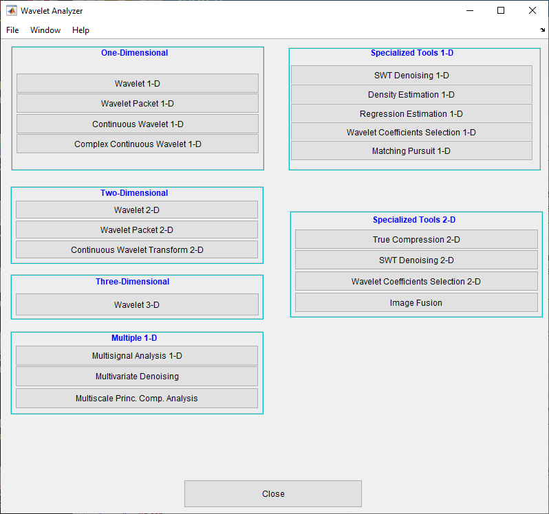

ClickMultivariate Denoisingto open theMultivariate Denoisingportion of the app.

Load data.

At the MATLAB command prompt, type

load ex4mwden

These signals are noisy versions from simple combinations of the two original signals. The first one is “Blocks” which is irregular and the second is “HeavySine” which is regular except around time 750. The other two signals are the sum and the difference between the original signals. Multivariate Gaussian white noise exhibiting strong spatial correlation is added to the resulting four signals.

The following example illustrates the two different aspects of the proposed denoising method. First, perform a convenient change of basis to cope with spatial correlation and denoise in the new basis. Then, use PCA to take advantage of the relationships between the signals, leading to an additional denoising effect.

Perform a wavelet decomposition and diagonalize the noise covariance matrix.

Use the displayed default values for theWavelet,DWT Extension Mode, and the decompositionLevel, and then clickDecompose and Diagonalize。The tool displays the wavelet approximation and detail coefficients of the decomposition of each signal in the original basis.

SelectNoise Adapted Basisto display the signals and their coefficients in the noise-adapted basis.

To see more information about this new basis, clickMore on Noise Adapted Basis。A new figure displays the robust noise covariance estimate matrix and the corresponding eigenvectors and eigenvalues.

Eigenvectors define the change of basis, and eigenvalues are the variances of uncorrelated noises in the new basis.

The multivariate denoising method proposed below is interesting if the noise covariance matrix is far from diagonal exhibiting spatial correlation, which, in this example, is the case.

denoise the multivariate signal.

A number of options are available for fine-tuning the denoising algorithm. However, we will use the defaults: fixed form soft thresholding, scaled white noise model, and the proposed numbers of retained principal components. In this case, the default values for PCA lead to retaining all the components.

SelectOriginal Basisto return to the original basis and then click消除干扰。

The results are satisfactory. Both of the two first signals are correctly recovered, but they can be improved by getting more information about the principal components. ClickMore on Principal Components。

SelectFile > Save denoised Signals。

SelectSave denoised Signals and Parameters。出现一个对话框that lets you specify a folder and filename for storing the signal.

Type the names_ex4mwdenand clickOKto save the data.

Load the variables into your workspace:

load s_ex4mwdent whos