Interpolation Methods

Interpolation估计是一个过程吗values that lie between known data points.

Interpolation involves the construction of a functionfthat matches givendata values,y_i, at givendatasites,x_i, in the sense thatf(x_i) =y_i, alli.

The interpolant,f, is usually constructed as the unique function of the form

$f (x) = \sum_{j} f_{j} (x) a_{j}$

that matches the given data, with the functionsf_jchosen “appropriately”.

In spline interpolation, one chooses thef_jto be thenconsecutive B-splinesB_j(x) =B(x|t_j,...,t_j+k),j= 1:n, of orderkfor some knot sequencet₁≤t₂≤ ... ≤t_n+k.

About Interpolation Methods

Method	Description
Linear	Linear interpolation. This method fits a different linear polynomial between each pair of data points for curves, or between sets of three points for surfaces.
Nearest neighbor	Nearest neighbor interpolation. This method sets the value of an interpolated point to the value of the nearest data point. Therefore, this method does not generate any new data points.
Cubic spline	Cubic spline interpolation. This method fits a different cubic polynomial between each pair of data points for curves, or between sets of three points for surfaces.
Shape-preserving	Piecewise cubic Hermite interpolation (PCHIP). This method preserves monotonicity and the shape of the data. For curves only.
Biharmonic (v4)	MATLAB^®4`griddata`method. For surfaces only.
Thin-plate spline	Thin-plate spline interpolation. This method fits smooth surfaces that also extrapolate well. For surfaces only.

For surfaces, the Interpolant fit type uses the MATLABscatteredInterpolantfunction for linear and nearest methods, and the MATLABgriddatafunction for cubic and biharmonic methods. The thin-plate spline method uses thetpapsfunction.

interpolant使用的类型取决于characteristics of the data being fit, the required smoothness of the curve, speed considerations, post-fit analysis requirements, and so on. The linear and nearest neighbor methods are fast, but the resulting curves are not very smooth. The cubic spline and shape-preserving and v4 methods are slower, but the resulting curves are very smooth.

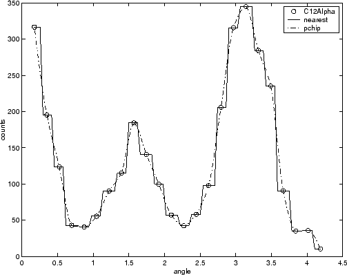
For example, the nuclear reaction data from thecarbon12alpha.matfile is shown here with a nearest neighbor interpolant fit and a shape-preserving (PCHIP) interpolant fit. Clearly, the nearest neighbor interpolant does not follow the data as well as the shape-preserving interpolant. The difference between these two fits can be important if you are interpolating. However, if you want to integrate the data to get a sense of the total strength of the reaction, then both fits provide nearly identical answers for reasonable integration bin widths.

Note

Goodness-of-fit statistics, prediction bounds, and weights are not defined for interpolants. Additionally, the fit residuals are always 0 (within computer precision) because interpolants pass through the data points.

Interpolants are defined aspiecewise polynomialsbecause the fitted curve is constructed from many “pieces” (except forBiharmonicfor surfaces which is a radial basis function interpolant). For cubic spline and PCHIP interpolation, each piece is described by four coefficients, which the toolbox calculates using a cubic (third-degree) polynomial.

Refer to thesplinefunction for more information about cubic spline interpolation.
Refer to thepchipfunction for more information about shape-preserving interpolation, and for a comparison of the two methods.
Refer to thescatteredInterpolant,griddata, andtpapsfunctions for more information about surface interpolation.

It is possible to fit a single “global” polynomial interpolant to data, with a degree one less than the number of data points. However, such a fit can have wildly erratic behavior between data points. In contrast, the piecewise polynomials described here always produce a well-behaved fit, so they are more flexible than parametric polynomials and can be effectively used for a wider range of data sets.

Interpolation Methods

About Interpolation Methods

Related Topics

Curve Fitting Toolbox Documentation

金宝app

Machine Learning Challenges: Choosing the Best Classification Model and Avoiding Overfitting